Stochastic versions of the alternating direction method of multiplier (ADMM) and its variants play a key role in many modern large-scale machine learning problems. In this work, we introduce a unified algorithmic framework called generalized stochastic ADMM and investigate their continuous-time analysis. The generalized framework widely includes many stochastic ADMM variants such as standard, linearized and gradient-based ADMM. Our continuous-time analysis provides us with new insights into stochastic ADMM and variants, and we rigorously prove that under some proper scaling, the trajectory of stochastic ADMM weakly converges to the solution of a stochastic differential equation with small noise. Our analysis also provides a theoretical explanation of why the relaxation parameter should be chosen between 0 and 2.
For modern industrial-scale machine learning problems, with the massive amount of data that are not only extremely large but often stored or even collected in a distributed manner, stochastic first-order methods almost become one of the default choices due to their excellent performance for the online streaming large-scale datasets. The stochastic version of the alternating direction method of multiplier (ADMM) algorithms is a popular approach to handling this distributed setting, especially for regularized empirical risk minimization. Consider the following stochastic optimization problem:

where  ) with
 ![]() ) as the loss incurred on a sample
) as the loss incurred on a sample  ,
,  , and both f and g are convex. The alternating direction method of multiplier (ADMM) [BPC
 ] rewrites (1.1) as a constrained optimization problem

Here and throughout the rest of the paper, we overload f to ease the notation, i.e. we adopt the two-argument ![]() ) for the stochastic instance and one-argument
) for the stochastic instance and one-argument ![]() ) for its expectation. Note the classical setting of linear constraint Ax + Bz = c can be reformulated as z = Ax by a linear transformation when B is invertible. In the batch learning setting, f(x) can be approximated by the empirical risk
) for its expectation. Note the classical setting of linear constraint Ax + Bz = c can be reformulated as z = Ax by a linear transformation when B is invertible. In the batch learning setting, f(x) can be approximated by the empirical risk  ). However, the computation cost for minimizing
  a large amount of samples is significantly high and the efficiency is limited under the time and resource constraints. In the stochastic setting, at each step
  is updated based on a small batch of samples (or even one)
 ![]() instead of a large batch or full batch.
instead of a large batch or full batch.
Introducing stochasticity to ADMM [BPC ] is in parallel to incorporating noise into gradient descent [WB12, Suz13, OHTG13]. At iteration k + 1, a sample
  is randomly drawn as an independent realization of
 ![]() . Analogous to stochastic gradient descent, our stochastic ADMM (sADMM ) introduced in [Suz13, OHTG13] performs the following updates:
. Analogous to stochastic gradient descent, our stochastic ADMM (sADMM ) introduced in [Suz13, OHTG13] performs the following updates:
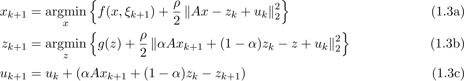
![]() 0 is called the penalty parameter [BPC
0 is called the penalty parameter [BPC ]. Here
 ![]() (0, 2) is introduced as a relaxation parameter [BPC
(0, 2) is introduced as a relaxation parameter [BPC ]. The algorithm is split into different regimes of
 ![]() as follows:
as follows:
• ![]()
• ![]() 1, corresponding to the over-relaxed stochastic ADMM ;
1, corresponding to the over-relaxed stochastic ADMM ;
• ![]() 1, corresponding to the under-relaxed stochastic ADMM.
1, corresponding to the under-relaxed stochastic ADMM.
Historically, the above relaxation schemes were introduced and analyzed in [EB92], and the experiments in [EF98] suggest that the over-relaxed regime of ![]() 1 can improve the convergence rate. The acceleration phenomenon in over-relaxed ADMM has been discussed from the continuous perspective in deterministic setting [YZLS19, FRV23], where relaxed the ADMM algorithm accelerates by a factor of
1 can improve the convergence rate. The acceleration phenomenon in over-relaxed ADMM has been discussed from the continuous perspective in deterministic setting [YZLS19, FRV23], where relaxed the ADMM algorithm accelerates by a factor of ![]() 2) in its convergence rate.
2) in its convergence rate.
Since the emergence of ADMM, many variants have been introduced recently for solving a variety of optimization tasks. We focus on two ADMM variants (in our stochastic setting) to cater to the need in application:
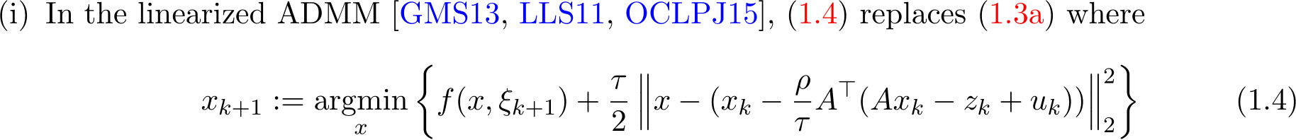
In words, the augmented Lagrangian function is approximated by linearizing the quadratic term of x in (1.3a) plus the addition of a proximal term 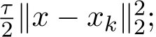

In words, instead of solving x-subproblem (1.3a) accurately, we apply one step of gradient descent with stepsize 1![]()
In this paper we formulate a general scheme, called Generalized stochastic ADMM (G-sADMM), to accommodate and unify all these variants of stochastic ADMM:
where the objective ![]() -subproblem is defined as
-subproblem is defined as
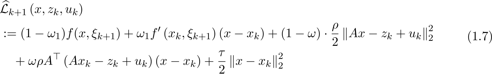
with parameter ![]() 2) and explicitness parameters
2) and explicitness parameters ![]()
We study the continuous-time limit of the stochastic sequence ![]() defined in (1.6a) as
defined in (1.6a) as ![]() . Following the recent line of work [FRV18] [FRV23] and [YZLS19], we adopt a (speed-up) time rescaling of
. Following the recent line of work [FRV18] [FRV23] and [YZLS19], we adopt a (speed-up) time rescaling of  , namely the stepsize for (stochastic) ADMM, and hence we are in the small-stepsize regime as in (stochastic) gradient descent. Also, the proximal parameter
 ![]() grows linearly in
grows linearly in ![]() . In our setting of continuous limit theory, we focus on a fixed interval by T (referred to as ”time”), corresponding to
. In our setting of continuous limit theory, we focus on a fixed interval by T (referred to as ”time”), corresponding to ![]() discrete steps (referred to as ”step”) in discrete time. Our main results can be concluded as follows:
discrete steps (referred to as ”step”) in discrete time. Our main results can be concluded as follows:
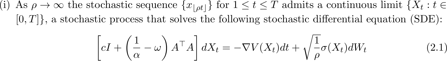
where we recall from (1.1) that V (x) = f(x) + g(Ax). The right hand of (2.1) consists of a deterministic part and a stochastic part, where ![]() ) is some diffusion matrix defined later in (3.8) and
) is some diffusion matrix defined later in (3.8) and  is the standard Brownian motion in
  The continuous-limit approximation
is rigorously characterized by weak convergence![]() in the sense that applying a test function
in the sense that applying a test function ![]() of a certain class, the expectation of
of a certain class, the expectation of 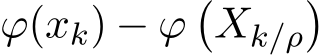 is uniformly in
 ![]() ] convergent to zero when
] convergent to zero when ![]() tends to infinity as stated in Theorem 3.
tends to infinity as stated in Theorem 3.![]() The above SDE carries the small parameter
The above SDE carries the small parameter in its diffusion term and is also called stochastic modified equation (SME) [LTE19], due to the historical reason in numerical analysis [Mil95, KP11].
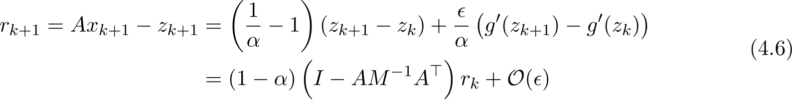
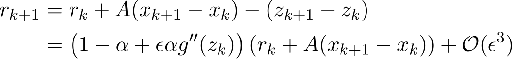
(ii) We provide a continuous-time explanation of the effect of relaxation parameter ![]() (0, 2) in stochastic ADMM, which is the first among stochastic ADMM work to our best knowledge. In light of our weak convergence of the discrete algorithm
(0, 2) in stochastic ADMM, which is the first among stochastic ADMM work to our best knowledge. In light of our weak convergence of the discrete algorithm  , the residual
  approximately satisfies
  (1
(1 ![]() and converges to 0 at a geometric rate
and converges to 0 at a geometric rate ![]() 1. The rigorous statement is in Corollary 5.
1. The rigorous statement is in Corollary 5.
2.1 Contributions
Our contribution to this paper is the first continuous-time analysis of stochastic ADMM. First, we present a unified stochastic differential equation as the continuous-time model of variants of stochastic ADMM (standard ADMM, linearized ADMM, gradient-based ADMM) in the regime of large ![]() weak convergence. By showing the effective dynamic is restricted in the x-component and a careful analysis of noisy fluctuation, we revealed that these stochastic ADMM variants surprisingly have the essentially same continuous limit and the exact diffusion terms as preconditioned SGD, regardless of the constraint, the distributed nature and the stochasticity as well as various parameters in consideration.
weak convergence. By showing the effective dynamic is restricted in the x-component and a careful analysis of noisy fluctuation, we revealed that these stochastic ADMM variants surprisingly have the essentially same continuous limit and the exact diffusion terms as preconditioned SGD, regardless of the constraint, the distributed nature and the stochasticity as well as various parameters in consideration.
Second, we characterize the time evolution of std( ) and std(
 ) in their continuous-time counterparts and explicitly show that the standard deviation of stochastic ADMM variants has the scaling
  in stochastic ADMM. Finally, our theoretical analysis of the continuous model provides a simple justification of the effect of relaxation parameter
 ![]() 2) and further sheds light on the principled choices of parameters
2) and further sheds light on the principled choices of parameters ![]()
2.2 Related work
ADMM is a widely used algorithm for solving problems with separable structures in machine learning, statistics, control, etc. ADMM has a close connection with operator-splitting methods [DR56, PR55, GM75]. But ADMM comes back to popularity due to several works like [CP07, GO09, WYYZ08] and the highly influential survey paper [BPC ]. Numerous modern machine learning applications are inspired by ADMM, for example, [NLR
![+15, MSD+18, YZ11, MSP+19, SYDB18, SB18, PL19].](https://cdn.bytez.com/mobilePapers/v2/arxiv/2404.14358/images/3-20.png) Linearized ADMM and gradient-based ADMM are widely used variants of ADMM. Linearized ADMM has been studied extensively, for example, in [CT94, HLHY02, LLS11, Ma16, Xu15, YY13, YZ11, ZBBO10, OCLPJ15]; gradient-based ADMM has been studied extensively too, for example, in [Con13, Vu13, DY17, LMZ17]. In this work, we present a general formulation for relaxed, linearized and gradient-based ADMM, and extended all of them to stochastic optimization.
Linearized ADMM and gradient-based ADMM are widely used variants of ADMM. Linearized ADMM has been studied extensively, for example, in [CT94, HLHY02, LLS11, Ma16, Xu15, YY13, YZ11, ZBBO10, OCLPJ15]; gradient-based ADMM has been studied extensively too, for example, in [Con13, Vu13, DY17, LMZ17]. In this work, we present a general formulation for relaxed, linearized and gradient-based ADMM, and extended all of them to stochastic optimization.
Several important works studied the relaxation scheme of ADMM [EB92, EF98] and propose to choose ![]() (0, 2) with the empirical suggestion for over relaxation 1
(0, 2) with the empirical suggestion for over relaxation 1 ![]() 2. In this work, we give a simple and elegant proof of the theoretical reason that
2. In this work, we give a simple and elegant proof of the theoretical reason that ![]() (0, 2). The recent work in [FRV18, FRV23] establishes the first deterministic continuous-time model for standard ADMM in the form of ordinary differential equation (ODE) for the smooth ADMM and [FRV23, YZLS19] extends its work to non-smooth ADMM, using the tool of differential inclusion, which is motivated by [VJFC18, ORX
(0, 2). The recent work in [FRV18, FRV23] establishes the first deterministic continuous-time model for standard ADMM in the form of ordinary differential equation (ODE) for the smooth ADMM and [FRV23, YZLS19] extends its work to non-smooth ADMM, using the tool of differential inclusion, which is motivated by [VJFC18, ORX ]. The use of stochastic and online techniques for ADMM has recently drawn a lot of interest. [WB12] first proposed the online ADMM, which learns from only one sample (or a small mini-batch) at a time. [OHTG13, Suz13] proposed the variants of stochastic ADMM to attack the difficult nonlinear optimization problem inherent in
 ![]() ) by linearization. Very recently, further accelerated algorithms for the stochastic ADMM have been developed in [ZK14, HCH19]. There are also recent works on combining variance reduction technique and stochastic ADMM [ZK16, LSC17, YH17]
) by linearization. Very recently, further accelerated algorithms for the stochastic ADMM have been developed in [ZK14, HCH19]. There are also recent works on combining variance reduction technique and stochastic ADMM [ZK16, LSC17, YH17]
The work in [SBC16] is one seminal work of using the continuous-time dynamical system to analyze discrete algorithms for optimization such as Nesterov’s accelerated gradient method, with important extension to high resolution and symplectic structure in [ACPR18, SDJS22, SDSJ19, Jor18, FJV21], to variational perspective in [WRJ21, WWJ16]. The mathematical analysis of continuous formulation for stochastic optimization algorithms has become an important trend in recent years. We select an under-represented list out of numerous works: analyzing SGD from the perspective of Langevin MCMC [ZLC17, CCBJ18, GGZ22, SSJ23], analyzing stochastic mirrordescent [ZMB ], analyzing the SGD for the online algorithm of specific statistical models [LWLZ17, LWL16, LTE17]. The mathematical connection between the stochastic gradient descent (SGD) and stochastic modified equation (SME) has been insightfully discovered in [LTE17, LTE19]. This SME technique, originally arising from the numerical analysis of SDE [Mil95, KP11], has become the major mathematical tool for stochastic or online algorithms. The idea of using optimal control for stochastic continuous models to find adaptive parameters like step-size for stochastic optimization is used in [LTE17] to control adaptive step size and momentum, and in [AWS
 ] to improve the control on momentum, in [HLLL19, FGL
 ] to choose batch size via diffusion approximation.
In this section, we show the weak approximation to the generalized family of stochastic ADMM variants (G-sADMM ) (1.6a)—(1.6c). Throughout this section, we define  to serve as an analog of stepsize for (stochastic) ADMM. The G-sADMM scheme (1.6a)—(1.6c) contains the relaxation parameter
 ![]() , the parameter
, the parameter ![]() and the implicitness parameters
and the implicitness parameters ![]() . This scheme (1.6a)—(1.6c) is very general and includes many existing variants as follows. It recovers all deterministic variants of ADMM for the setting
. This scheme (1.6a)—(1.6c) is very general and includes many existing variants as follows. It recovers all deterministic variants of ADMM for the setting ![]() ). If
). If ![]() — (1.6c) is the standard stochastic ADMM (sADMM ) or online ADMM [OHTG13, ZK14]. For the setting of parameters
— (1.6c) is the standard stochastic ADMM (sADMM ) or online ADMM [OHTG13, ZK14]. For the setting of parameters ![]() 0 it becomes stochastic version of the linearized ADMM for acceleration [HLHY02, ZBBO10, OCLPJ15]. If
0 it becomes stochastic version of the linearized ADMM for acceleration [HLHY02, ZBBO10, OCLPJ15]. If  0, this scheme is the stochastic version of the gradient-based ADMM [Con13, Vu13, DY17, LMZ17]. In addition, the stochastic ADMM considered in [OHTG13] for non-smooth function corresponds to the setting here with
3.1 Stochastic differential equations, weak approximation, and stochastic modified equations
In this subsection, we introduce several basic concepts, including the definition of stochastic differential equations, the weak approximation, and the stochastic modified equations. Let  be the standard Wiener process (i.e. Brownian motion) in
  . An equation of the form
![]()
where b(x, t) :  and
and ![]() ) :
) :  are given mappings and
  is an unknown stochastic process, is called a stochastic differential equation (SDE). In (3.1), vector field b is the drift coefficient, matrix
 ![]() is the
is the ![]() is the
is the ![]()
![]() on any interval [0, T] can be heuristically regarded as the limit of the stochastic differential equation
on any interval [0, T] can be heuristically regarded as the limit of the stochastic differential equation  with
with  as
as ![]() 0 and
0 and ![]()
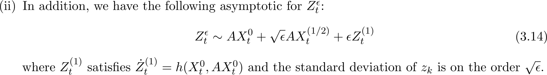
On the other hand, for any Markov process  with a continuous path, if the limits b(x, t) := lim
![h↓0 1hE [Xt+h − Xt | Xt = x] and Σ(x, t) := limh↓0 1hE�(Xt+h − Xt)(Xt+h − Xt)⊤ | Xt = x�exist,](https://cdn.bytez.com/mobilePapers/v2/arxiv/2404.14358/images/5-18.png) then the Markov process
then the Markov process  satisfies an SDE given by (3.1) as its weak solution. The weak solution roughly refers to the distributions sense in contrast to the realiaations of the path. We next state the weak convergence below. For any
 ![]() 1, if a uniform bound on the p-th moments holds, then the weak convergence is equivalent to the convergence in the Wasserstein-p metric.
1, if a uniform bound on the p-th moments holds, then the weak convergence is equivalent to the convergence in the Wasserstein-p metric.
Definition 1 (Weak convergence). We say the family (parametrized by ![]() ) of the stochastic sequence
) of the stochastic sequence  0, weakly converges to (or is a weak approximation to) a family of continuous-time Ito processes
 ![]() :
:  with the order p if they satisfy the following condition: For any time interval T > 0 and for any test function
 ![]() and its partial derivatives up to order 2p + 2 belong to F, there exists a constant
and its partial derivatives up to order 2p + 2 belong to F, there exists a constant  0 such that for any
 ![]()

The constant  in the above inequality are independent of
 ![]() but may depend on T and
but may depend on T and ![]() . In the classic applications to the numerical method for SDE [Mil95], the continuous solution
. In the classic applications to the numerical method for SDE [Mil95], the continuous solution ![]() is usually independent of
is usually independent of ![]() ; for the stochastic modified equation,
; for the stochastic modified equation, ![]() does depend on
does depend on ![]() . We drop the subscript
. We drop the subscript  for notational ease whenever there is no ambiguity.
The idea of using the weak approximation and the stochastic modified equation was rigorously carried out in [LTE17], which is based on an important theorem due to [Mil86]. In brief, Milstein’s theorem links the one-step difference, which has been detailed above, to the global approximation in the weak sense, by checking three conditions on the momentums of the one-step difference. Since we only consider the first-order weak approximation, Milstein’s theorem is introduced in a simplified form below for only p = 1. The more general situations can be found in Theorem 5 in [Mil86], Theorem 9.1 in [Mil95] and Theorem 14.5.2 in [KP11].
Let the stochastic sequence ![]() be recursively defined by the iteration written in the form associated with a function
be recursively defined by the iteration written in the form associated with a function ![]()
![]()
where ![]() are i.i.d. random variables. The initial
are i.i.d. random variables. The initial  , and we define the one step difference ¯∆
  . We use the parenthetical subscript to denote the dimensional components of a vector like ¯∆
  ). Assume that there exists a function
 ![]() such that ¯∆ satisfies the bounds of the fourth momentum
such that ¯∆ satisfies the bounds of the fourth momentum

for any component indices  , For any arbitrary
 ![]() 0, consider the family of the Ito processes
0, consider the family of the Ito processes  defined by a stochastic differential equation whose noise depends on the parameter
 ![]()
![]()
 is the standard Wiener process in
  . The initial is
  . The coefficient functions b and
 ![]() satisfy certain standard Lipschitz and linear growth conditions; see [Mil95, LTE19]. Define
satisfy certain standard Lipschitz and linear growth conditions; see [Mil95, LTE19]. Define ![]() for the SDE (3.5).
for the SDE (3.5).
Theorem 2 (Milstein’s weak convergence theorem). If there exists a constant  and a function
 ![]() , such that the following conditions of the first three moments on the error ∆
, such that the following conditions of the first three moments on the error ∆ 
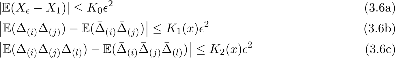
hold for any ![]() and any
and any  , then
 ![]() weakly converges to
weakly converges to ![]() with the order 1. In light of the above theorem, we will now call (3.5) the stochastic modified equation (SME) of the iterative scheme (3.3).
with the order 1. In light of the above theorem, we will now call (3.5) the stochastic modified equation (SME) of the iterative scheme (3.3).
For the SDE (3.5) at the small noise ![]() , by the Ito-Taylor expansion, it is wellknown that
, by the Ito-Taylor expansion, it is wellknown that  for all integer
 ![]() 3 and the component index
3 and the component index ![]() . For more we refer to [KP11] and Lemma 1 in [LTE17]. Hence the main receipt to apply Milstein’s theorem is to examine the conditions of the momentums for the discrete sequence ¯
. For more we refer to [KP11] and Lemma 1 in [LTE17]. Hence the main receipt to apply Milstein’s theorem is to examine the conditions of the momentums for the discrete sequence ¯
One prominent work [LTE17] is to use the SME as a weak approximation to understand the dynamical behavior of the stochastic gradient descent (SGD). The prominent advantage of this technique is that the fluctuation in the SGD iteration can be well captured by the fluctuation in the SME. We brief the result as follows. For the expectation minimization problem min![]()
 ), the SGD iteration is
 ![]() with the step size
with the step size ![]() . Then by Theorem 2, the corresponding SME of first-order approximation is
. Then by Theorem 2, the corresponding SME of first-order approximation is
![]()
with  . Details can be found in [LTE17]. The SGD here is analogous to the forward-time Euler-Maruyama approximation since
 ![]()
3.2 Main results
We introduce some notations and assumptions. We use ![]() to denote the Euclidean two norm if the subscript is not specified. All vectors are referred to as column vectors.
to denote the Euclidean two norm if the subscript is not specified. All vectors are referred to as column vectors. ![]() ) and
) and ![]() ) refer to the first (gradient) and second (Hessian) derivatives w.r.t. x. The first assumption is Assumption I : f(x), g and for each
) refer to the first (gradient) and second (Hessian) derivatives w.r.t. x. The first assumption is Assumption I : f(x), g and for each ![]() ), are closed proper convex functions; A has full column rank.
), are closed proper convex functions; A has full column rank.
Let F be the set of functions of at most polynomial growth. To apply the SME theory, we need the following Assumption II on the smoothness:
(i) The second order derivative ![]() are uniformly bounded in x, and almost surely in
are uniformly bounded in x, and almost surely in ![]() for
for  is uniformly bounded in x;
![]()
(iii) ![]() ) satisfy a uniform growth condition:
) satisfy a uniform growth condition: ![]() constant C independent of
constant C independent of ![]()
The conditions (ii) and (iii) are inherited from [Mil86], which can be relaxed to a certain extent without compromising the conclusion here. For instance, the linear growth condition of the gradient in (iii) is only needed on a compact domain. Refer to [LTE19] for technical and rigorous improvement for these assumptions on f.
With the prior notations and assumptions in hand, we present our first main theorem as follows. Given the noisy gradient ![]() ) and its expectation
) and its expectation  ), we define the following covariance matrix

We conclude
Theorem 3 (SME for G-sADMM). Let ![]() (0, 2),
(0, 2), ![]() and
and ![]() 0. Let
0. Let  (0
(0![]() denote the sequence of stochastic ADMM (1.6a)—(1.6c) with the initial choice
denote the sequence of stochastic ADMM (1.6a)—(1.6c) with the initial choice  Define
  as a stochastic process satisfying the SDE

where the matrix

Figure 1: The match between the stochastic ADMM and the SME and the verification of the first-order weak approximation. The result is based on the average of 10![]() independent runs: step size
independent runs: step size ![]() 5 in (b). The details can be referred to in Section 5.
5 in (b). The details can be referred to in Section 5.
Then we have 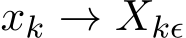 in weak convergence of order 1, with the following precise meaning: for any time interval T > 0 and for any test function
 ![]() such that
such that ![]() and its partial derivatives up to order 4 belong to F, there exists a constant C such that
and its partial derivatives up to order 4 belong to F, there exists a constant C such that
![]()
Remark 4. The stochastic scheme (1.6a)—(1.6c) is the simplest form of using only one instance of the gradient ![]() ) in each iteration. If a batch size larger than one is used, then the one instance gradient
) in each iteration. If a batch size larger than one is used, then the one instance gradient ![]() ) is replaced by the average
) is replaced by the average 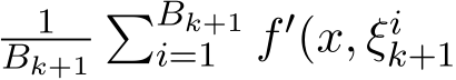 ) where
  1 is the batch size and (
 ) are
) are  i.i.d. samples. Under these settings, Σ should be multiplied by a fact
  where the continuous-time function
  is the linear interpolation of
  at times
  . The stochastic modified equation (3.9) is then in the following form
 ![]()
The proof of the theorem (as long as the upcoming results) is delegated to the next section. Here we highlight one useful corollary resulting from our proof of the theorem.
Corollary 5. For generalized stochastic ADMM, when ![]() , the residual
, the residual  the relation:
 ![]() ). So, the necessary condition on the relaxation parameter
). So, the necessary condition on the relaxation parameter ![]() for the residual convergence
for the residual convergence 
![]()
This corollary matches the empirical range ![]() (0, 2) proposed for standard ADMM with relaxation [BPC
(0, 2) proposed for standard ADMM with relaxation [BPC![+11].](https://cdn.bytez.com/mobilePapers/v2/arxiv/2404.14358/images/8-26.png)
As an illustration of Theorem 3 for the first order weak convergence, Figure 1b verifies this rate for various ![]() and even different g. To show that the SME does not only provide the expectation of the solution but also provides the fluctuation of the numerical solution
and even different g. To show that the SME does not only provide the expectation of the solution but also provides the fluctuation of the numerical solution  for any given
 ![]() plots the match of mean and standard deviation of
plots the match of mean and standard deviation of  from the SME versus the
  from the sADMM. Section 5 includes more examples and tests for understanding the role of stochastic fluctuation and the relaxation parameter.
Base on (3.9) in Theorem 3, the simple asymptotic expansion for small ![]() immediately shows that the standard deviation of the stochastic ADMM
immediately shows that the standard deviation of the stochastic ADMM  is
is  ) and the rescaled two standard deviations
  ) and
) and  ) are close as the functions of the time
  . The upcoming Section 3.3 discusses this issue and other conclusions on the continuous dynamics of the
  variable satisfying
 ![]()
3.3 Continuous dynamics of zk
Based on the SME (3.9), we can find the stochastic asymptotic expansion of  fixed interval [0, T]

See Chapter 2 in [FW12] for rigorous justification.  is deterministic as the gradient flow of the deterministic problem: ˙
 ),
),  and
and  are stochastic and satisfy certain SDEs independent of
 ![]() . The useful conclusion is that the standard deviation of
. The useful conclusion is that the standard deviation of  , mainly coming from the term
  ). Hence, the standard deviation of
  from the stochastic ADMM is also
  ) and the rescaled two standard deviations
  ) and
) and  ) are close as the functions of the time
We can further investigate the fluctuation of the sequence  generated by the stochastic ADMM and the modified equation of its continuous version
Theorem 6. We have

such that ![]() is a weak approximation to
is a weak approximation to ![]() with the order 1, where
with the order 1, where  is the solution to the SME (3.9).
We may consider a special case where 
![]()
Recall the residual  and in view of (4.15), we have the following result that there exists a function

and the residual ![]() is a weak approximation to
is a weak approximation to ![]() with the order 1. If
with the order 1. If ![]() sADMM (1.6a)—(1.6c), then the expectation and standard deviation of
sADMM (1.6a)—(1.6c), then the expectation and standard deviation of  are both at order
  ). If
). If ![]() —(1.6c), then the expectation and standard deviation of
—(1.6c), then the expectation and standard deviation of  are only at order
 ![]()
We provide the proof of our main results in this section.
Proof regarding SME for G-sADMM, Theorem 3. The ADMM scheme is the iteration of the triplet (![]() . In our proof, we shall show this triplet iteration can be effectively reduced to the iteration of x variable only in the form of
. In our proof, we shall show this triplet iteration can be effectively reduced to the iteration of x variable only in the form of ![]() ). The main approach for this reduction is the analysis of the residual
). The main approach for this reduction is the analysis of the residual  below. This one step
  will play a central role in the theory of weak convergence, Milstein’s theorem (Theorem 2 in Section 3.1) [Mil86].
For notational ease, we drop the random variable  in the scheme (1.6a)—(1.6c); the readers bear in mind that f and its derivatives do involve
 ![]() and all conclusions hold almost surely for
and all conclusions hold almost surely for ![]()
The optimality conditions for the scheme (1.6a)—(1.6c) are
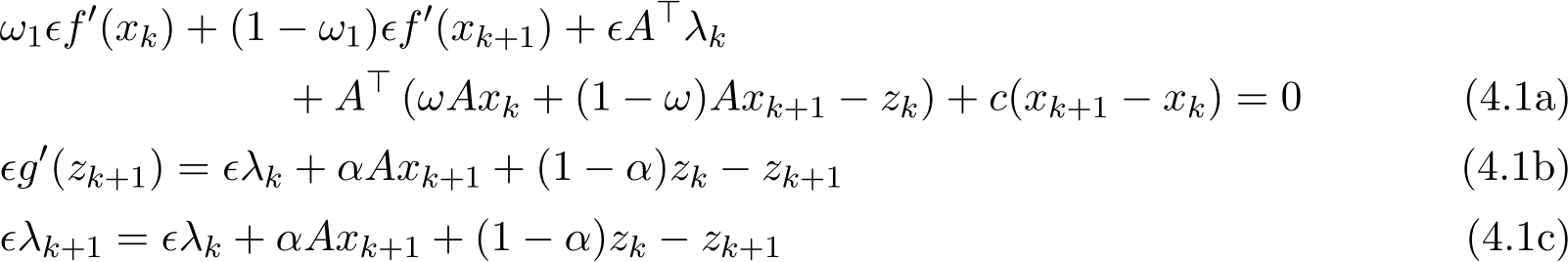
Note that due to (4.1b) and (4.1c), the last condition (4.1c) can be replaced by ![]() ). So, without loss of generality, one can assume that
). So, without loss of generality, one can assume that
![]()
for any integer k. The optimality conditions (4.1a)—(4.1c) now can be written only in the pair (x, z):
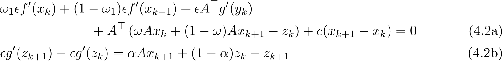
We treat (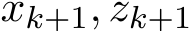 ) in (4.2a)—(4.2b) as a function of
 ![]() and
and ![]() and seek the asymptotic expansion of this function in the regime of small
and seek the asymptotic expansion of this function in the regime of small ![]() , by using Dominant Balance technique (see, e.g. [Whi10]) with the Taylor expansion for
, by using Dominant Balance technique (see, e.g. [Whi10]) with the Taylor expansion for ![]() ) and
) and ![]() ) around
) around  and
and  , respectively. The expansion of the one-step difference up to the order
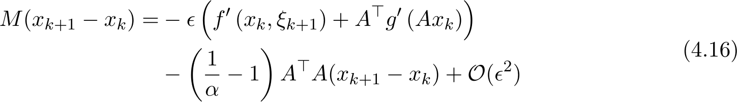
 ![]()
where 
![]()
and the matrix M is

![]() is a matrix depending on the hessian
is a matrix depending on the hessian  are uniformly bounded in k (and in random element
 ![]() ) due to the bound of functions
) due to the bound of functions ![]() and
and ![]() in Assumption II. Throughout the rest of the paper, we shall use the notation
in Assumption II. Throughout the rest of the paper, we shall use the notation ![]() ) to denote these terms bounded by a (nonrandom) constant multiplier of
) to denote these terms bounded by a (nonrandom) constant multiplier of ![]()
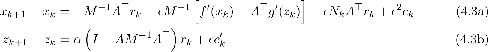
(4.3a)—(4.3b) clearly shows that the dynamics of the pair (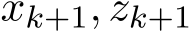 ) depends on the residual
  in the previous step. In the limit of
 ![]()
 which does not vanish unless
  tends to zero. We turn to the analysis of the residual. (4.3b) together with (4.3a) implies

by absorbing all ![]() order terms into
order terms into ![]() ). By using (4.2b) for
). By using (4.2b) for  , we have the recursive relation for residual
Since ![]() , (4.6) shows that
, (4.6) shows that ![]() become
become ![]() ) after one iteration.
) after one iteration.
Next, we have the following important property, particularly with assumption ![]() stronger result than (4.6).
stronger result than (4.6).
Proposition 7. For any integer ![]()

If ![]() ) reduces to the second order in
) reduces to the second order in ![]()

Proof of Proposition 7. Since ![]() ), then the one step difference
), then the one step difference  and
and 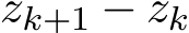 are both at order
 ![]() ) because of (4.3a) and (4.3b). We solve
) because of (4.3a) and (4.3b). We solve ![]() by linearizing the implicit term
by linearizing the implicit term ![]() ) and use the assumption that the third order derivative of g exits:
) and use the assumption that the third order derivative of g exits:

where ![]() ). Then since
). Then since  ), the expansion of
  from the above equation leads to

Together with the definition of  , the above suggests
concluding the proposition.
We now focus on (4.3a) for  , which can be rewritten as
This expression does not contain the parameter ![]() explicitly, but the residual
explicitly, but the residual ![]() significantly depends on
significantly depends on ![]() (see Proposition 7). If
(see Proposition 7). If ![]() is on the order of
is on the order of  , which leads to the useful fact that there is no contribution from
  to the weak approximation of
  at the order 1. But for the relaxation case where
 ![]() contains the first order term coming from
contains the first order term coming from 
To obtain a second order for some ”residual” for the relaxed scheme where ![]() new definition,
new definition, ![]() -residual, to account for the gap induced by
-residual, to account for the gap induced by ![]() . Motivated by (4.1b), we first define
. Motivated by (4.1b), we first define
![]()
It is connected to the original residual  since it is easy to check that

Obviously, when  is the original residual
 ![]() . In our proof, we need a modified
. In our proof, we need a modified ![]() -residual, denoted by
-residual, denoted by
![]()
We shall show that both  are as small as

In fact, by the second equality of (4.12), (4.9) becomes 
 ), so
), so  ) (
) ( ) which is
  ) since
 ![]() ).
).
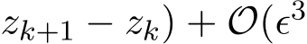
Figure 2: Illustration of the order of the residual  defined in (4.11).
The difference between (![]() , is at the order
, is at the order  due to truncation error of the central difference scheme. Then we have the conclusion
and it follows 
Remark 8. As an illustration, the figure above for a toy example (see numerical example part in Section 5) shows that  regardless of
 ![]() (the solid lines are
(the solid lines are  and the dashed lines are
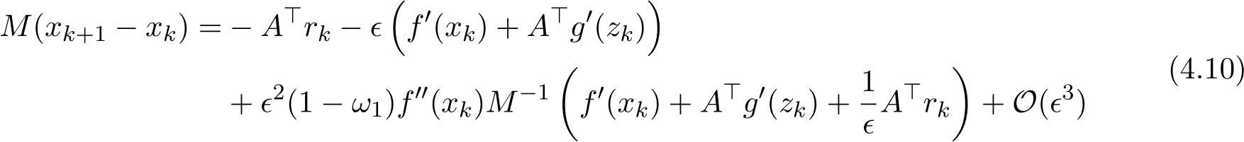
With the above preparations for the residual analysis, we now apply Theorem 2 to show the main conclusion of our theorem. Combining (4.10) and (4.15), and noting the Taylor expansion of ![]() ), and now putting back the random element
), and now putting back the random element ![]()
For convenience, introduce the matrix

and let ![]()

The final step is to compute the momentums and verify the conditions in Milstein’s theorem (Theorem 2) on these momentums. We have
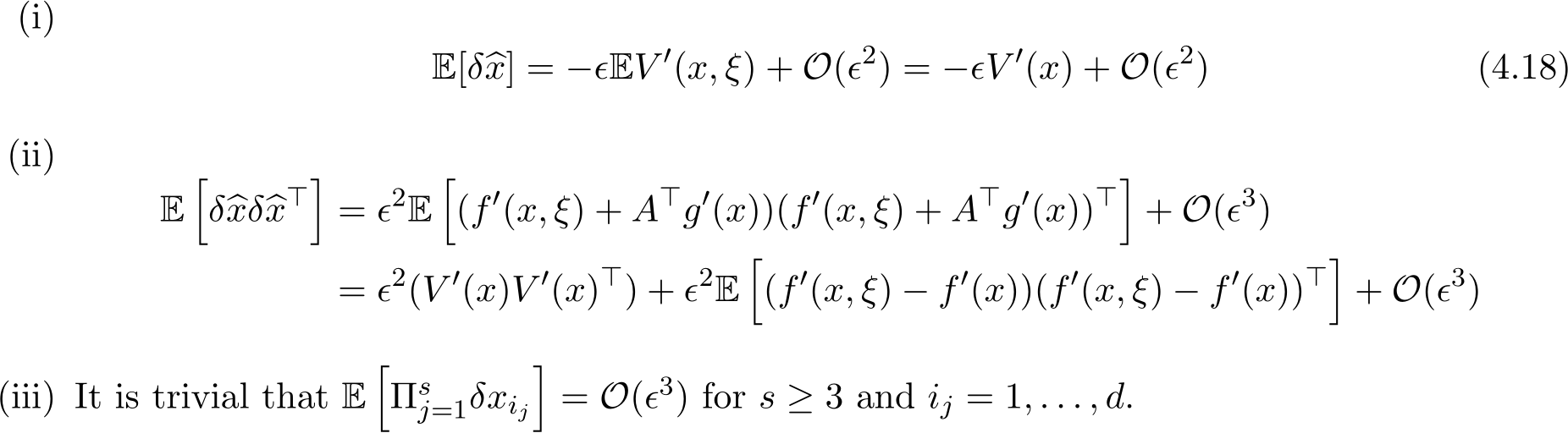
This in all completes the proof of Theorem 3.
![]()
Remark 9. We do not pursue the second-order weak approximation as for the SGD scheme, due to the complicated issue of the residuals. In addition, the proof requires a regularity condition for the functions f and g. So, our theoretic theorems can not cover the non-smooth function g. Our numerical tests in Section 5 suggest that the conclusion holds too for  regularization function
 ![]()
Remark 10. In general applications, it can be difficult to obtain the explicit expression of the covariance matrix Σ(x) as a function of x, except in very few simplified cases. In applications of empirical risk minimization, the function f is the empirical average of the loss on each sample  ). The diffusion’s covariance matrix Σ(x) in (3.8) becomes the following form

It is clear that if ![]() i.i.d. samples
i.i.d. samples ![]()
Proof of Corollary 5 Based on Proposition 7,

Since ![]() are bounded and
are bounded and ![]() ), then
), then ![]() ), with the leading term (1
), with the leading term (1 ![]() . Therefore when
. Therefore when ![]() , we need
, we need ![]() 1 for
1 for  to converge to zero. This completes the proof.
![]()
Proof of Theorem 6 (4.15) and (4.3b) indicate that

Therefore ˙ +
+ ![]() . The function h is deterministic because the update of
. The function h is deterministic because the update of  in (4.2b) is deterministic conditioned on the given
  . The function h depends on
 ![]() and others, which is quite challenging to obtain the explicit expression, completing the proof.
and others, which is quite challenging to obtain the explicit expression, completing the proof.
![]()
We show some remarks first to elaborate our main theorem in practical settings before we present our illustrative examples.
In empirical risk minimization problems, the function f is the empirical average of the loss on each sample  ). The diffusion matrix Σ(x) in (3.8) can be written as the following:

If ![]() ) with N i.i.d. samples
) with N i.i.d. samples ![]() , then Σ
, then Σ![]() Σ(x) as
Σ(x) as ![]() . In addition, the stochastic scheme (1.6a)—(1.6c) uses only one instance of the gradient
. In addition, the stochastic scheme (1.6a)—(1.6c) uses only one instance of the gradient ![]() ) in each iteration. Under cases where more than one samples are computed in each iteration, then the one instance gradient
) in each iteration. Under cases where more than one samples are computed in each iteration, then the one instance gradient ![]() ) is replaced by the batch gradient
) is replaced by the batch gradient  batch size and (
 ) are
) are  i.i.d. samples. Under these settings, Σ should be multiplied by a factor
  where the continuous-time function
  is the linear interpolation of
  at times
  . The stochastic modified equation (3.9) is then of the following form

5.1 A toy example
In (1.2), consider  is a Bernoulli random variable taking values
 ![]() 1 or +1 with equal probability. For g(z) we consider both of the cases of
1 or +1 with equal probability. For g(z) we consider both of the cases of 
and g(z) = |z|, and we fix the matrix A = I. Recall in the stochastic ADMM (1.6a)—(1.6c), ![]() and
and ![]() [0, 1]. We choose
[0, 1]. We choose  . When
  , the optimum solution of (1.2) is
  16374 and the SME is

It is easy to verify that these settings satisfy the assumptions in our main theorem. Throughout the analyses below, we also numerically investigated the convergence rate for the non-smooth penalty g(z) = |z|, even though this  regularization function does not satisfy our
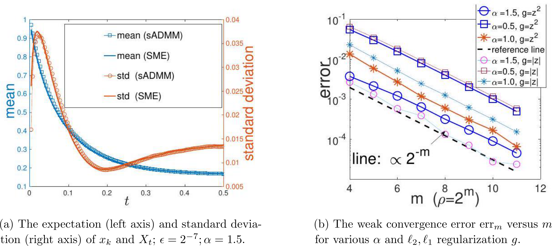
Figure 3: The match between the stochastic ADMM and the SME and the verification of the first-order weak approximation. The result is based on the average of 10![]() independent runs. The step size
independent runs. The step size ![]() 5 in (b). The details can be referred to in Section 5.
5 in (b). The details can be referred to in Section 5.
assumptions in theory. For the corresponding SDE, formally we can write

by using the sign function for ![]() ). We only use the above SME for this simulation. The rigorous expression requires the concept of stochastic differential inclusion, which is out of the scope of this work.
). We only use the above SME for this simulation. The rigorous expression requires the concept of stochastic differential inclusion, which is out of the scope of this work.
We initialize ![]() ) and set the terminal time as T = 0.5.
) and set the terminal time as T = 0.5.
Convergence between generalized stochastic ADMM and its continuous model. First of all, we verify that the SME solution not only provides the approximation of the expectation of the G-sADMM (1.6a)—(1.6c) solution, but also depicts the fluctuation of the numerical solution  of (1.6a)—(1.6c) for any given
 ![]() . In Figure 1a we compare the mean and standard deviation (”std”) between
. In Figure 1a we compare the mean and standard deviation (”std”) between  and
and  for
for  and under
  as an illustration of our argument. The left vertical axis together with two blue curves depicts the means of the two solution paths and the right vertical axis with two red curves are the standard deviations of the two solution paths respectively. We see from Figure 1a that both the mean curves of the SME/GsADMM and the std curves of the SME/GsADMM coincide with each other.
In Figure 1b we plot the order of weak convergence in Theorem 3. We choose a test function  to evaluate the weak convergence error:
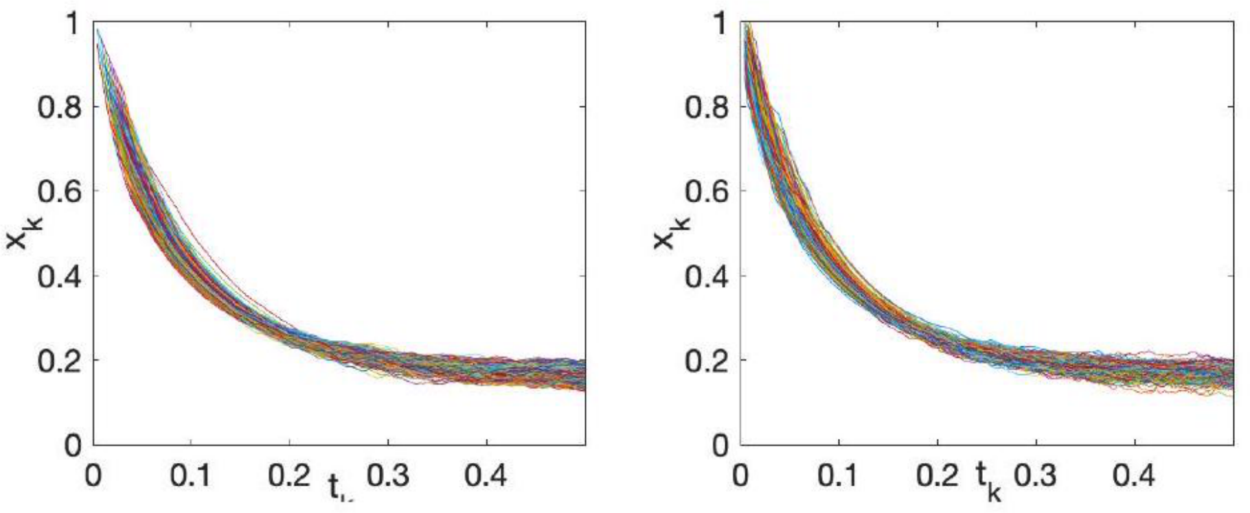
Figure 4: The 400 sample trajectories from stochastic ADMM (left) and SME (right).
For each m = 4, 5, . . . , 11, we set ![]() and
and ![]() . We plot m as the x-axis and err
. We plot m as the x-axis and err![]() as the y-axis in Figure 1b and apply the semi-log scale for both three values of relaxation parameter
as the y-axis in Figure 1b and apply the semi-log scale for both three values of relaxation parameter ![]() and two cases of g(z). We see that err
and two cases of g(z). We see that err![]() satisfies (3.11) in Theorem 3 and thus verifies the weak convergence of order one.
satisfies (3.11) in Theorem 3 and thus verifies the weak convergence of order one.
In addition, we plot 400 sample trajectories of the GsADMM together in Figure 4, left panel and 400 sample trajectories of the SME together in Figure 4, right panel, with  and
and ![]() 5. This further shows the match between the mean and the std between the solution paths of the stochastic ADMM and the SME.
5. This further shows the match between the mean and the std between the solution paths of the stochastic ADMM and the SME.
![]() In Figure 5, we explore how
In Figure 5, we explore how ![]() affects and accelerate the optimization of the stochastic ADMM (1.6a)—(1.6c). The continuous model (5.3) supports this observation here that a large
affects and accelerate the optimization of the stochastic ADMM (1.6a)—(1.6c). The continuous model (5.3) supports this observation here that a large ![]() helps fast decay toward the true minimizer. Similar effects have been described for the deterministic ADMM in [YZLS19].
helps fast decay toward the true minimizer. Similar effects have been described for the deterministic ADMM in [YZLS19].
 Next, we test the orders of the standard deviation of
  and
and  . Previously in Section 3.3 (see (3.12) and (3.14)), we mentioned that theoretically the standard deviation of the sequences
  and
and  are of order
 ![]() . So the two sequences
. So the two sequences 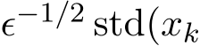 ) and
) and 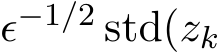 ) should only depends on
 ![]() regardless of
regardless of ![]() , which is shown in Figure 6.
, which is shown in Figure 6.
![]() Finally, note that Proposition 7 in the proof of Theorem 3 and its continuous counterpart (3.15) in Section 3.3 indicate that the residual
Finally, note that Proposition 7 in the proof of Theorem 3 and its continuous counterpart (3.15) in Section 3.3 indicate that the residual  is
is  both its expectation and its standard deviation. Figure 7 plots the two quantities
 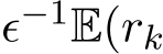 ) and
) and  to verify that both
  are of order
  when
when  ) and
) and  ) to show that both
  and std
  are
are
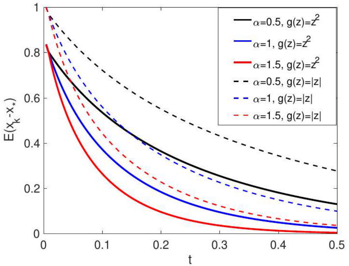
Figure 5: The expectation of the error to true minimizer ![]() 2) varies. The result is based on the average of 10000 runs of stochastic ADMM sequences.
2) varies. The result is based on the average of 10000 runs of stochastic ADMM sequences.
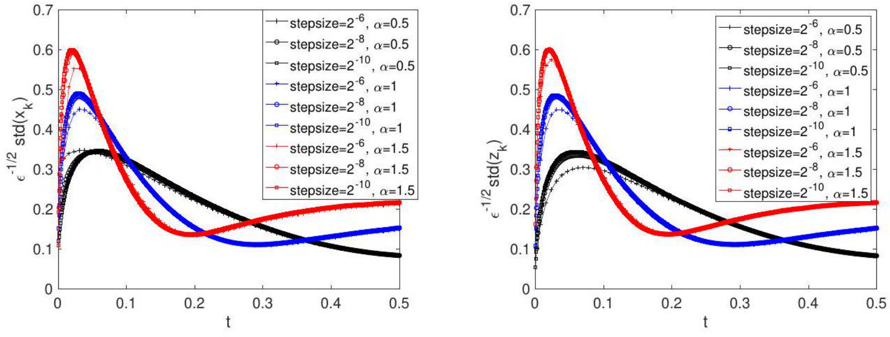
Figure 6: The rescaled std of 
of order  . Moreover, as mentioned in Remark 8, the new definition of the residual,
  is
is  ) regardless of
 ![]() , as confirmed numerically by Figure 8.
, as confirmed numerically by Figure 8.
5.2 Generalized ridge and lasso regression
In this subsection, we perform experiments on the generalized ridge/lasso regression:
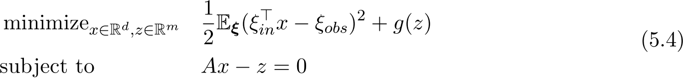
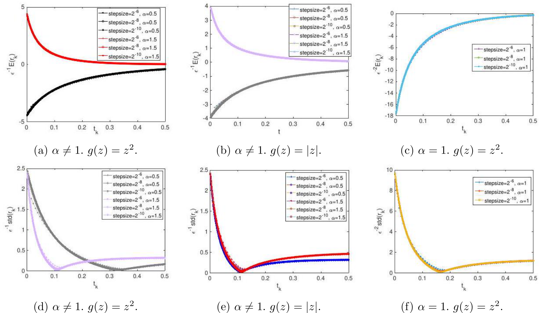
Figure 7: The scaling of the mean (first row) and std (second row) of residual  : for
: for ![]() are on the order
are on the order 
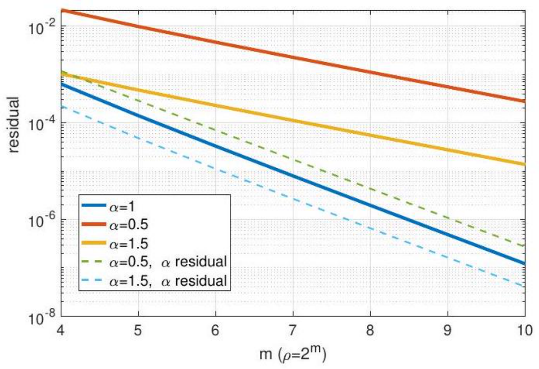
Figure 8: Illustration of the order of the residual  defined in (4.11).
where 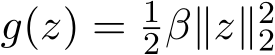 (ridge regression) or
 ![]() (lasso regression), with a constant
(lasso regression), with a constant ![]() 0. A is a penalty matrix specifying the desired structured pattern of x. Among the random variables
0. A is a penalty matrix specifying the desired structured pattern of x. Among the random variables 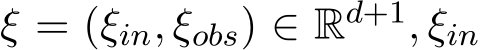 is a zero-mean random (column) vector uniformly distributed over the hyper-cube [
![−0.5, 0.5]d](https://cdn.bytez.com/mobilePapers/v2/arxiv/2404.14358/images/19-10.png) with independent components. The labelled output data
with independent components. The labelled output data  , where
  is a known vector and
 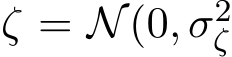 ) is the zero-mean measurement noise which is independent of
 ![]() . For this regression problem, we have
. For this regression problem, we have
 . Thus,
  and
and ![]() ) The true solution of the ridge regression with
) The true solution of the ridge regression with  is
is 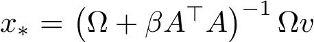 . The analytic expression of the diffusion matrix Σ(x) can be written in terms of the fourth-order momentum of the stochastic vector
 ![]()

As mentioned at the beginning of this Section 5, we can use a batch size B for the stochastic ADMM. Then the corresponding SME (5.2) for the ridge regression problem is

The stochastic modified differential inclusion for the lasso regression (formally) is

To solve these SDEs, the main computational bottleneck is the computation of the matrix Σ(x). We can reduce this overhead by using a sample version for the covariance matrix Σ(x) as shown (5.1). At each ![]() ) is computed by N samples of the random
) is computed by N samples of the random ![]() . A small N has a large gain in computational efficiency with the potential negative impact on the accuracy. However, our extensive numerical tests show that even for a small N, the weak approximation of
. A small N has a large gain in computational efficiency with the potential negative impact on the accuracy. However, our extensive numerical tests show that even for a small N, the weak approximation of  is still extraordinarily good. N = 9 is used for our results reported here when the numerical solution of the SME is involved.
In our experiments, we set the dimension d = 3. Let A be the Hilbert matrix multiplied by 0.5. Note that ![]() is quite close to singular since the minimal eigenvalue is only 1.8e
is quite close to singular since the minimal eigenvalue is only 1.8e![]() 6. Set
6. Set  2 and set the vector v as linspace(1, 2, d). Choose the initial
  as the zero vector,
 ![]()
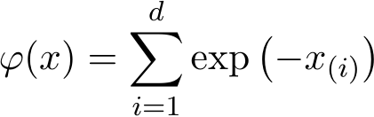
for ridge regression, which is the sum of all components. For the lasso regression, we choose the objective function f(x) + g(Ax) as the test function:

since the optimal solution is not unique. The choice of the step size ![]() integer m.
integer m.
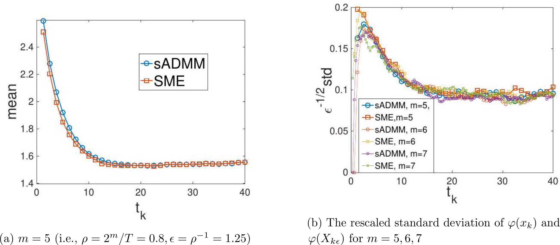
Figure 9: The mean and standard deviation of ![]() ) (sADMM) and
) (sADMM) and ![]()
 . The results are based on 400 independent runs.
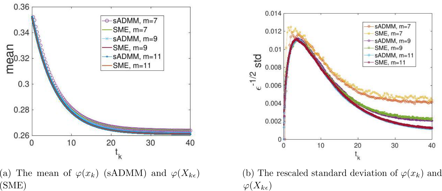
Figure 10: The mean and standard deviation of ![]() ) (sADMM) and
) (sADMM) and ![]()
 . The results are based on 4000 independent runs.
Consistence between G-sADMM and SME. We show in Figure 9a the mean of ![]() ) and
) and ![]() ) versus the time
) versus the time  , for a moderately large
 ![]() 25 at
25 at ![]() is as small as 0.8). The results agree very well even for this small
is as small as 0.8). The results agree very well even for this small ![]() 1. To test the match of the fluctuation, we plot in Figure 9b the rescaled standard deviation,
1. To test the match of the fluctuation, we plot in Figure 9b the rescaled standard deviation,  std, from both the stochastic ADMM and the continuous model for three different values of
 ![]() 7. This figure confirms the scaling of std is
7. This figure confirms the scaling of std is  ) and the weak convergence between the
  . It is worth pointing out
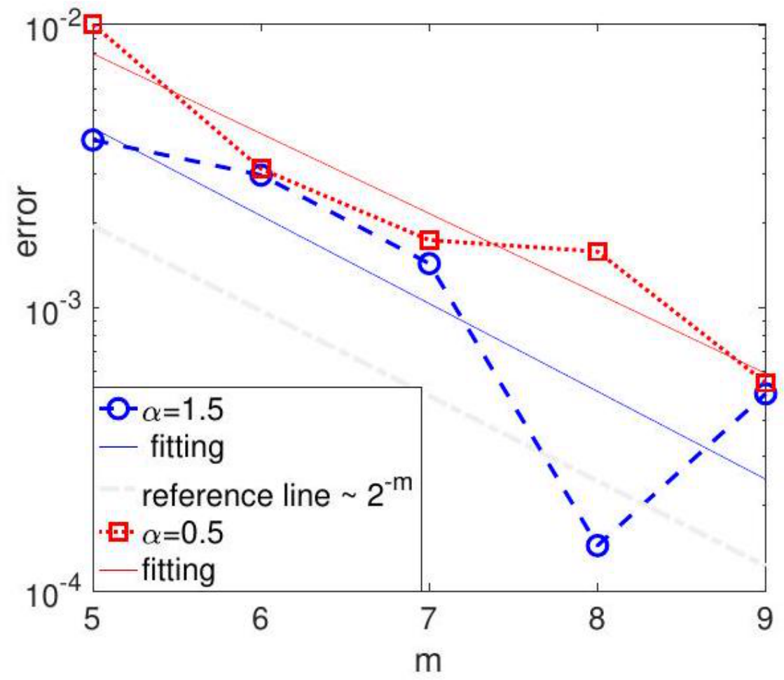
Figure 11: The weak convergence of order 1. The error is![��E[φ(x⌊Tρ⌋) − φ(XT )]��](https://cdn.bytez.com/mobilePapers/v2/arxiv/2404.14358/images/22-1.png) . Ridge regression. 4000 independent runs. Other parameters are the same as in Figure 9;
. Ridge regression. 4000 independent runs. Other parameters are the same as in Figure 9; ![]() . The reference line has the exact slope
. The reference line has the exact slope ![]() 1 in the semi-log plot, corresponding to the exact relation that error
1 in the semi-log plot, corresponding to the exact relation that error ![]()
Figure 12: With the fixed ![]() 5, the convergence/divergence of
5, the convergence/divergence of  from stochastic ADMM for
 ![]() . The average and standard deviation of the error
. The average and standard deviation of the error ![]() are based on 400 independent runs.
are based on 400 independent runs. 
 15 (less than the critical value 0
![]()
M has one negative eigenvalue ![]() 0153 and the ADMM trajectory
0153 and the ADMM trajectory ![]()
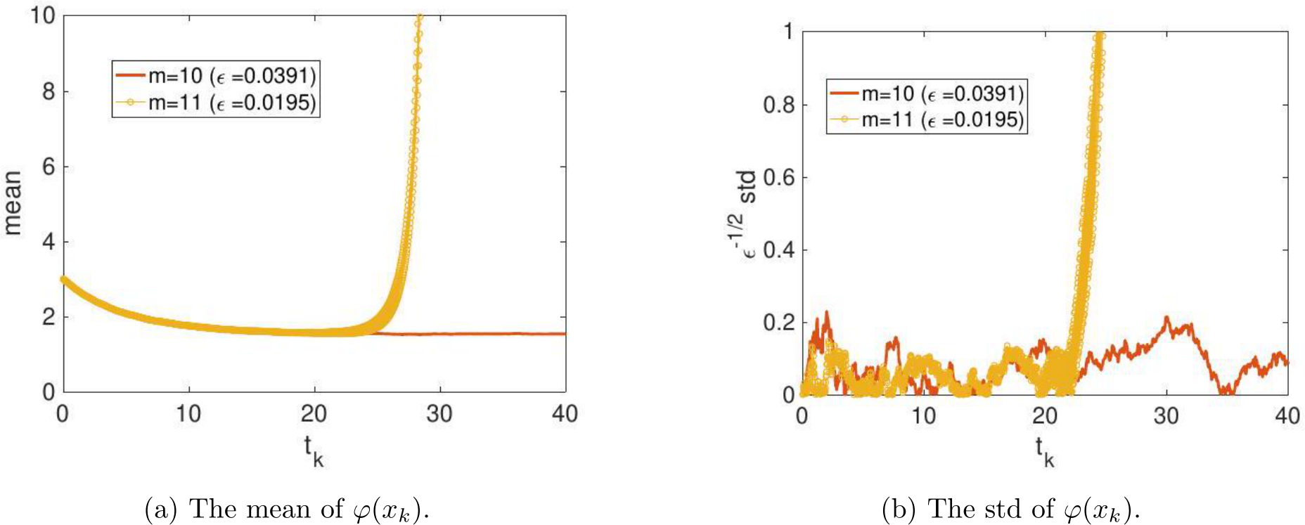
Figure 13: ![]() 02. The trajectory
02. The trajectory  from stochastic ADMM almost surely diverges if the stepsize
 ![]() is small enough.
is small enough. ![]() 400 independent runs. T = 40.
400 independent runs. T = 40.
that the values of ![]() are not large, only 0.8, 1.6, 3.2, even though in the weak convergence, the limit of
are not large, only 0.8, 1.6, 3.2, even though in the weak convergence, the limit of ![]() is considered in Theorem 3.
is considered in Theorem 3.
The results for lasso regression are also shown in Figure 10, where we see the agreement for the means from stochastic ADMM and the SME and the agreement of the standard deviations for any fixed ![]() . This suggests that Theorem 3 may hold too even for non-smooth g. However, the (rescaled) standard deviations for different
. This suggests that Theorem 3 may hold too even for non-smooth g. However, the (rescaled) standard deviations for different ![]() do not overlap, so the scaling of std(
do not overlap, so the scaling of std( ) is
) is  ) may break down, in the case of a non-smooth g.
Weak convergence. The numerical verification of the weak convergence is presented in Figure 11 for the ridge regression, where g is smooth and satisfies the regularity assumption in our theory.
![]() Recall
Recall ![]() , so c determines the choice of the parameter
, so c determines the choice of the parameter ![]() used in G-sADMM (1.6a)—(1.6c). Note
used in G-sADMM (1.6a)—(1.6c). Note ![]() + (1
+ (1![]() plays the important role in the SME (3.9).
plays the important role in the SME (3.9).
![]() (1, 2). Figure 12a studies the behavior of convergence towards the true minimum point
(1, 2). Figure 12a studies the behavior of convergence towards the true minimum point  with the over-relaxation
 ![]() 5. Then for
5. Then for ![]() stops being positive definite when c < 0.165; while for
stops being positive definite when c < 0.165; while for ![]() is always positive definite for any c > 0. Figure 12 a shows the consistency of the convergence with the positive definiteness of
is always positive definite for any c > 0. Figure 12 a shows the consistency of the convergence with the positive definiteness of  Figure 12b shows the standard deviation when c varies. Our observation here for the over-relaxation is that a smaller c can help decay faster (acceleration) on the expectation, but the fluctuation in stochastic ADMM also rises. Figure 12b at large time (t > 20) suggests that when the solution approaches the equilibrium (i.e., in saturation), the fluctuation is then independent of the choice of c.
![]()
![]() For the under-relaxation, 1
For the under-relaxation, 1![]() 1] and thus
1] and thus ![]() is always positive definite, whose smallest eigenvalue is very close to c. However, we observed in tests that
is always positive definite, whose smallest eigenvalue is very close to c. However, we observed in tests that  diverges regardless of how small
 ![]() is less than 0.16. For sufficient large
is less than 0.16. For sufficient large ![]() converges. This suggests there are some myths about the convergence in this under-relaxation case:
converges. This suggests there are some myths about the convergence in this under-relaxation case:
M should be stronger than positive definite with some small but strictly positive lower bound for the eigenvalues to ensure the convergence. Our current Corollary 5 and the continuous model in Theorem 3 are insufficient to answer this myth, which will be a future work.
![]() (0, 2). In addition, for any negative
(0, 2). In addition, for any negative ![]() or
or ![]() 2, the stochastic ADMM scheme always diverges if
2, the stochastic ADMM scheme always diverges if ![]() is sufficiently small (i.e.
is sufficiently small (i.e. ![]() is sufficiently large), which is in alignment with Corollary 5 about the asymptotics of residual in the small
is sufficiently large), which is in alignment with Corollary 5 about the asymptotics of residual in the small ![]() regime: the residual converges to zero if and only if
regime: the residual converges to zero if and only if ![]() (0, 2). It is important to note that if
(0, 2). It is important to note that if ![]() is not small enough, the ADMM sequence may also converge for
is not small enough, the ADMM sequence may also converge for ![]() (0, 2). As an illustration, we set
(0, 2). As an illustration, we set ![]() 02 and compute the stochastic ADMM with two different stepsize
02 and compute the stochastic ADMM with two different stepsize ![]() shows that for the smaller stepsize, the stochastic ADMM actually diverges since the corresponding continuous model is not stable.
shows that for the smaller stepsize, the stochastic ADMM actually diverges since the corresponding continuous model is not stable.
5.3 Discussion on adaptive parameter adjustment for step size, batch size, c and
![]()
We showed above the SME formulation for understanding the dynamics of the stochastic ADMM both in theory and in numerics. We now turn to a more interesting and challenging issue of how Theorem 3 can help design better adaptive schemes in practice. In general, the main idea is based on some optimal control problem for the derived continuous-time model [LTE17]. The seek of the solvable and simple results of underlying control problems is the main endeavor to make the algorithm work efficiently in practice. We here mainly focus on the one-dimensional case d = 1 to present the idea and the extension to high dimensional problems might be carried out by imposing a local diagonal-quadratic assumption.
Two-phase behavior. The two-phase behavior of training convex functions with stochastic gradient is well known [MB11, LTE17]. The transition time  is defined by the time when
  , the descent dominates and after
  , the fluctuation dominates. For a solvable SDE, as an illustration, we consider
  +
+ ![]() , which gives
, which gives 
![]()
Adaptive batch size. The stochastic scheme (1.6a)—(1.6c) uses only one instance of the gradient ![]() ) in each iteration. If
) in each iteration. If ![]() ) is replaced by the average
) is replaced by the average 
 1 is the batch size and (
 ) are
) are  i.i.d. samples, then Σ should be multiplied by a factor
  where the continuous-time function
  is the linear interpolation of
  at times
  . The stochastic modified equation (3.9) is then in the following form
 ![]()
 . We consider the solvable SDE above again, but with adaptive
 . Then before
  , we can use a constant
  . After time
  , our goal is to control the fluctuation
 by increasing
  to be as small as
 ![]() . For the solvable SDE, this leads to the choice of
. For the solvable SDE, this leads to the choice of 
![]()
![]() The adaptive step size
The adaptive step size ![]() can be linear interpolated to a continuous-time step size
can be linear interpolated to a continuous-time step size  written in the form of
  where
where  is the maximal possible step size with a fixed
This step size adaptivity is exactly equivalent to the adaptive choice of ![]() with a fixed
with a fixed 

The adaptive choice of  can be implemented by the adaptive choice for the ADMM parameters
 ![]() and relaxation parameter
and relaxation parameter 
Our goal is to find an adaptive control rule of  to solve min
![u:[0,T]→[0,1] EV (XT )](https://cdn.bytez.com/mobilePapers/v2/arxiv/2404.14358/images/25-24.png) subject to (5.5). We consider a one dimensional quadratic objective function
subject to (5.5). We consider a one dimensional quadratic objective function  and assume that
 ![]() a positive constant. The optimal control for this problem in the feedback form is
a positive constant. The optimal control for this problem in the feedback form is  [LTE17, FR75]. This policy means that if the fluctuation
  is small
compared to the objective value 2![]() ) (in the early stage of training), then
) (in the early stage of training), then  reaches its ceiling 1 and we use the minimal
  . To construct the minimal
  , one can set
 ![]() (or additionally
(or additionally ![]() we should use a larger
we should use a larger  . Increasing
  can be done by increasing c or decreasing
 ![]() (or
(or ![]() preferred). The feedback control
preferred). The feedback control  , after being plugged back in (3.9), leads to the open-loop result
  and consequently
 ![]() when
when  . Note in
a special case ![]() and the schedule for
and the schedule for ![]()
In this paper, we have developed the stochastic continuous dynamics in the form of a stochastic modified equation (SME) to analyze the dynamics of a general family of stochastic ADMM, including the standard, linearized and gradient-based ADMM with relaxation ![]() . Our continuous model (3.9) provides a unified framework to describe the dynamics of stochastic ADMM algorithms and particularly can quantify the fluctuation effect for a large penalty parameter
. Our continuous model (3.9) provides a unified framework to describe the dynamics of stochastic ADMM algorithms and particularly can quantify the fluctuation effect for a large penalty parameter ![]() . Our analysis here generalizes the existing works [FRV18, YZLS19] limited in ordinary differential equation, and reveals the impact of the noise in the stochastic ADMM. As the first-order approximation to the stochastic ADMM trajectory, the solution to the continuous model can precisely describe the mean and the standard deviation (fluctuation) of stochastic trajectories generated by stochastic ADMM.
. Our analysis here generalizes the existing works [FRV18, YZLS19] limited in ordinary differential equation, and reveals the impact of the noise in the stochastic ADMM. As the first-order approximation to the stochastic ADMM trajectory, the solution to the continuous model can precisely describe the mean and the standard deviation (fluctuation) of stochastic trajectories generated by stochastic ADMM.
One distinctive feature between the ADMM and its stochastic or online variants is highly similar to that between gradient descent and stochastic gradient descent [MB11, LTE17, SZ13]: there exists a transition time  after which the fluctuation (with a typical scale
  ) starts to dominate the ”drift” term, which means the traditional acceleration methods in deterministic case will fail to perform well, despite of their prominent performance in the early stage of training when the drift suppresses the noise. Our Section 5.3 extensively discusses this issue and the various aspects of the potential practicality of our theory: we briefly discuss a few new adaptive strategies such as for parameters
 ![]() , the batch size
, the batch size  and even relaxation parameters
  . For example, a large
 ![]() (over-relaxation) is preferred before the transition time while a small
(over-relaxation) is preferred before the transition time while a small ![]() (under-relaxation) may be preferred later to help reduce the variance.
(under-relaxation) may be preferred later to help reduce the variance.
For the possible further development in theory, we first note that we require the differential function f and g in our current assumption. With the tool of stochastic differential inclusion and set-value stochastic process [Kis03], we may also justify the given stochastic differential equation to allow the non-smooth g. In addition, our family of ADMM methods is still restricted to the linearized ADMM and the gradient-based ADMM. Recently, there emerge many new efficient acceleration methods for stochastic ADMM [PL19, ZK14, HCH19, OHTG13] and the stochastic variation reduction gradient in the context of ADMM [ZK16, LSC17, YH17]. A potential future work might be to extend our stochastic analysis to these broad families for a better understanding of their properties at the continuous level.
[ACPR18] Hedy Attouch, Zaki Chbani, Juan Peypouquet, and Patrick Redont. Fast convergence of inertial dynamics and algorithms with asymptotic vanishing viscosity. Mathematical Programming, 168:123–175, 2018.
[AWS![+18]](https://cdn.bytez.com/mobilePapers/v2/arxiv/2404.14358/images/26-5.png) Wangpeng An, Haoqian Wang, Qingyun Sun, Jun Xu, Qionghai Dai, and Lei Zhang. A PID controller approach for stochastic optimization of deep networks. In Proceedings of the IEEE conference on computer vision and pattern recognition, pages 8522–8531, 2018.
Wangpeng An, Haoqian Wang, Qingyun Sun, Jun Xu, Qionghai Dai, and Lei Zhang. A PID controller approach for stochastic optimization of deep networks. In Proceedings of the IEEE conference on computer vision and pattern recognition, pages 8522–8531, 2018.
[BPC![+11]](https://cdn.bytez.com/mobilePapers/v2/arxiv/2404.14358/images/26-6.png) Stephen Boyd, Neal Parikh, Eric Chu, Borja Peleato, Jonathan Eckstein, et al. Distributed optimization and statistical learning via the alternating direction method of multipliers.
Stephen Boyd, Neal Parikh, Eric Chu, Borja Peleato, Jonathan Eckstein, et al. Distributed optimization and statistical learning via the alternating direction method of multipliers. ![]() , 3(1):1–122, 2011.
, 3(1):1–122, 2011.
[CCBJ18] Xiang Cheng, Niladri S Chatterji, Peter L Bartlett, and Michael I Jordan. Underdamped Langevin MCMC: A non-asymptotic analysis. In Conference on learning theory, pages 300–323. PMLR, 2018.
[Con13] L. Condat. A primal-dual splitting method for convex optimization involving Lipschitzian, proximable and linear composite terms. J. Optimization Theory and Applications, 158(2):460–479, 2013.
[CP07] P. L. Combettes and Jean-Christophe Pesquet. A Douglas-Rachford splitting approach to nonsmooth convex variational signal recovery. IEEE Journal of Selected Topics in Signal Processing, 1(4):564–574, 2007.
[CT94] G. Chen and M. Teboulle. A proximal-based decomposition method for convex minimization problems. Math. Program., 64:81–101, 1994.
[DR56] J. Douglas and H. H. Rachford. On the numerical solution of the heat conduction problem in 2 and 3 space variables. Trans. Am. Math Soc., 82:421–439, 1956.
[DY17] D. Davis and W. Yin. A three-operator splitting scheme and its optimization applications. Set-Valued and Variational Analysis, 25(4):829–858, 2017.
[EB92] Jonathan Eckstein and Dimitri P Bertsekas. On the Douglas–Rachford splitting method and the proximal point algorithm for maximal monotone operators. Math. Program., 55(1-3):293–318, 1992.
[EF98] Jonathan Eckstein and Michael C Ferris. Operator-splitting methods for monotone affine variational inequalities, with a parallel application to optimal control. INFORMS J. on Comput., 10(2):218–235, 1998.
[FGL![+20]](https://cdn.bytez.com/mobilePapers/v2/arxiv/2404.14358/images/27-0.png) Yuanyuan Feng, Tingran Gao, Lei Li, Jian-Guo Liu, and Yulong Lu. Uniform-in-time weak error analysis for stochastic gradient descent algorithms via diffusion approximation. Communications in Mathematical Sciences, 18(1), 2020.
Yuanyuan Feng, Tingran Gao, Lei Li, Jian-Guo Liu, and Yulong Lu. Uniform-in-time weak error analysis for stochastic gradient descent algorithms via diffusion approximation. Communications in Mathematical Sciences, 18(1), 2020.
[FJV21] Guilherme Fran¸ca, Michael I Jordan, and Ren´e Vidal. On dissipative symplectic integration with applications to gradient-based optimization. Journal of Statistical Mechanics: Theory and Experiment, 2021(4):043402, 2021.
[FR75] W H Fleming and R W Rishel. Deterministic and Stochastic Optimal Control. Springer New York, 1975.
[FRV18] Guilherme Fran¸ca, Daniel P Robinson, and Ren´e Vidal. ADMM and accelerated ADMM as continuous dynamical systems. In International Conference on Machine Learning, pages 1559–1567. PMLR, 2018.
[FRV23] Guilherme Fran¸ca, Daniel P Robinson, and Ren´e Vidal. A nonsmooth dynamical systems perspective on accelerated extensions of ADMM. IEEE Transactions on Automatic Control, 68(5):2966–2978, 2023.
[FW12] M. I. Freidlin and A. D. Wentzell. Random Perturbations of Dynamical Systems. Springer-Verlag, 2012.
[GGZ22] Xuefeng Gao, Mert G¨urb¨uzbalaban, and Lingjiong Zhu. Global convergence of stochastic gradient hamiltonian monte carlo for nonconvex stochastic optimization: Nonasymptotic performance bounds and momentum-based acceleration. Operations Research, 70(5):2931–2947, 2022.
[GM75] Daniel Gabay and Bertrand Mercier. A dual algorithm for the solution of non linear variational problems via finite element approximation. Institut de recherche d’informatique et d’automatique, 1975.
[GMS13] Donald Goldfarb, Shiqian Ma, and Katya Scheinberg. Fast alternating linearization methods for minimizing the sum of two convex functions. Math. Program., 141(1-2):349– 382, 2013.
[GO09] T. Goldstein and S. Osher. The split Bregman method for L1-regularized problems. SIAM J. Imaging Sci., 2:323–343, 2009.
[HCH19] Feihu Huang, Songcan Chen, and Heng Huang. Faster stochastic alternating direction method of multipliers for nonconvex optimization. In International Conference on Machine Learning, volume 97, pages 2839–2848, 2019.
[HLHY02] B. S. He, L. Liao, D. Han, and H. Yang. A new inexact alternating direction method for monotone variational inequalities. Math. Program., 92:103–118, 2002.
[HLLL19] Wenqing Hu, Chris Junchi Li, Lei Li, and Jian-Guo Liu. On the diffusion approximation of nonconvex stochastic gradient descent. Annals of Mathematical Sciences and Applications, 4(1), 2019.
[Jor18] Michael I Jordan. Dynamical, symplectic and stochastic perspectives on gradient-based optimization. University of California, Berkeley, 2018.
[Kis03] Michal Kisielewicz. Stochastic Differential Inclusions and Applications. Springer, 2003.
[KP11] P.E. Kloeden and E. Platen. Numerical Solution of Stochastic Differential Equations. Springer, New York, 2011.
[LLS11] Zhouchen Lin, Risheng Liu, and Zhixun Su. Linearized alternating direction method with adaptive penalty for low-rank representation. In Advances in Neural Information Processing Systems, pages 612–620, 2011.
[LMZ17] T. Lin, S. Ma, and S. Zhang. An extragradient-based alternating direction method for convex minimization. Foundations of Computational Mathematics, 17(1):35–59, 2017.
[LSC17] Yuanyuan Liu, Fanhua Shang, and James Cheng. Accelerated variance reduced stochastic ADMM. In Proceedings of the AAAI conference on artificial intelligence, page 2287, 2017.
[LTE17] Qianxiao Li, Cheng Tai, and Weinan E. Stochastic modified equations and adaptive stochastic gradient algorithms. In International Conference on Machine Learning, pages 3306–3340, 1 2017.
[LTE19] Qianxiao Li, Cheng Tai, and Weinan E. Stochastic modified equations and dynamics of stochastic gradient algorithms I: Mathematical foundations. Journal of Machine Learning Research, 20(40):1–47, 2019.
[LWL16] Chris Junchi Li, Zhaoran Wang, and Han Liu. Online ICA: Global dynamics of nonconvex optimization via diffusion processes. In Advances in Neural Information Processing Systems, pages 4967–4975, 2016.
[LWLZ17] Chris Junchi Li, Mengdi Wang, Han Liu, and Tong Zhang. Diffusion approximations for online principal component estimation and global convergence. In Advances in Neural Information Processing Systems, 2017.
[Ma16] S. Ma. Alternating proximal gradient method for convex minimization. J. Sci. Comput., 68(2):546–572, 2016.
[MB11] Eric Moulines and Francis Bach. Non-asymptotic analysis of stochastic approximation algorithms for machine learning. Advances in neural information processing systems, 24, 2011.
[Mil86] G. N. Milstein. Weak approximation of solutions of systems of stochastic differential equations. Theory of Probability & Its Applications, 30(4):750–766, 1986.
[Mil95] G.N. Milstein. Numerical Integration of Stochastic Differential Equations, volume 313. Springer, 1995.
[MSD![+18]](https://cdn.bytez.com/mobilePapers/v2/arxiv/2404.14358/images/29-0.png) Morteza Mardani, Qingyun Sun, David Donoho, Vardan Papyan, Hatef Monajemi, Shreyas Vasanawala, and John Pauly. Neural proximal gradient descent for compressive imaging. In Advances in Neural Information Processing Systems, pages 9596–9606, 2018.
Morteza Mardani, Qingyun Sun, David Donoho, Vardan Papyan, Hatef Monajemi, Shreyas Vasanawala, and John Pauly. Neural proximal gradient descent for compressive imaging. In Advances in Neural Information Processing Systems, pages 9596–9606, 2018.
[MSP![+19]](https://cdn.bytez.com/mobilePapers/v2/arxiv/2404.14358/images/29-1.png) Morteza Mardani, Qingyun Sun, Vardan Papyan, Shreyas Vasanawala, John Pauly, and David Donoho. Degrees of freedom analysis of unrolled neural networks. arXiv:1906.03742, 2019.
Morteza Mardani, Qingyun Sun, Vardan Papyan, Shreyas Vasanawala, John Pauly, and David Donoho. Degrees of freedom analysis of unrolled neural networks. arXiv:1906.03742, 2019.
[NLR![+15]](https://cdn.bytez.com/mobilePapers/v2/arxiv/2404.14358/images/29-2.png) Robert Nishihara, Laurent Lessard, Ben Recht, Andrew Packard, and Michael Jordan. A general analysis of the convergence of ADMM. In International conference on machine learning, pages 343–352. PMLR, 2015.
Robert Nishihara, Laurent Lessard, Ben Recht, Andrew Packard, and Michael Jordan. A general analysis of the convergence of ADMM. In International conference on machine learning, pages 343–352. PMLR, 2015.
[OCLPJ15] Yuyuan Ouyang, Yunmei Chen, Guanghui Lan, and Eduardo Pasiliao Jr. An accelerated linearized alternating direction method of multipliers. SIAM J. IMAGING SCI., 8(1):644–681, 2015.
[OHTG13] Hua Ouyang, Niao He, Long Tran, and Alexander Gray. Stochastic alternating direction method of multipliers. In International Conference on Machine Learning, volume 28, pages 80–88, 17–19 Jun 2013.
[ORX![+16]](https://cdn.bytez.com/mobilePapers/v2/arxiv/2404.14358/images/29-3.png) Stanley Osher, Feng Ruan, Jiechao Xiong, Yuan Yao, and Wotao Yin. Sparse recovery via differential inclusions. Applied and Computational Harmonic Analysis, 41(2):436–469, 2016.
Stanley Osher, Feng Ruan, Jiechao Xiong, Yuan Yao, and Wotao Yin. Sparse recovery via differential inclusions. Applied and Computational Harmonic Analysis, 41(2):436–469, 2016.
[PL19] Clarice Poon and Jingwei Liang. Trajectory of alternating direction method of multipliers and adaptive acceleration. In Advances in Neural Information Processing Systems, pages 7357–7365. 2019.
[PR55] D. H. Peaceman and H. H. Rachford. The numerical solution of parabolic elliptic differential equations. SIAM Journal on Applied Mathematics, 3:28–41, 1955.
[SB18] Qingyun Sun and Stephen Boyd. Distributional robust Kelly gambling. arXiv:1812.10371, 2018.
[SBC16] Weijie Su, Stephen Boyd, and Emmanuel Candes. A differential equation for modeling Nesterov’s accelerated gradient method: Theory and insights. Journal of Machine Learning Research, 17(153):1–43, 2016.
[SDJS22] Bin Shi, Simon S Du, Michael I Jordan, and Weijie J Su. Understanding the acceleration phenomenon via high-resolution differential equations. Mathematical Programming, pages 1–70, 2022.
[SDSJ19] Bin Shi, Simon S Du, Weijie Su, and Michael I Jordan. Acceleration via symplectic discretization of high-resolution differential equations. In Advances in Neural Information Processing Systems, pages 5745–5753, 2019.
[SSJ23] Bin Shi, Weijie Su, and Michael I Jordan. On learning rates and Schr¨odinger operators. Journal of Machine Learning Research, 24(379):1–53, 2023.
[Suz13] Taiji Suzuki. Dual averaging and proximal gradient descent for online alternating direction multiplier method. In International Conference on Machine Learning, pages 392–400, 2013.
[SYDB18] Qingyun Sun, Mengyuan Yan, David Donoho, and Stephen Boyd. Convolutional imputation of matrix networks. In International Conference on Machine Learning, pages 4818–4827. PMLR, 2018.
[SZ13] Ohad Shamir and Tong Zhang. Stochastic gradient descent for non-smooth optimization: Convergence results and optimal averaging schemes. In International Conference on Machine Learning, pages 71–79, 2013.
[VJFC18] Apidopoulos Vassilis, Aujol Jean-Fran¸cois, and Dossal Charles. The differential inclusion modeling FISTA algorithm and optimality of convergence rate in the case ![]() Journal on Optimization, 28(1):551–574, 2018.
Journal on Optimization, 28(1):551–574, 2018.
[Vu13] B. C. Vu. A splitting algorithm for dual monotone inclusions involving cocoercive operators. Advances in Computational Mathematics, 38(3):667–681, 2013.
[WB12] Huahua Wang and Arindam Banerjee. Online alternating direction method. In International Conference on Machine Learning, page 1699–1706, 10 2012.
[Whi10] Roscoe B White. Asymptotic Analysis of Differential Equations. Imperial College Press, 2010.
[WRJ21] Ashia C Wilson, Ben Recht, and Michael I Jordan. A Lyapunov analysis of accelerated methods in optimization. Journal of Machine Learning Research, 22(113):1–34, 2021.
[WWJ16] Andre Wibisono, Ashia C Wilson, and Michael I Jordan. A variational perspective on accelerated methods in optimization. proceedings of the National Academy of Sciences, 113(47):E7351–E7358, 2016.
[WYYZ08] Y. Wang, J. Yang, W. Yin, and Y. Zhang. A new alternating minimization algorithm for total variation image reconstruction. SIAM J. Imaging Sci., 1(3):248–272, 2008.
[Xu15] Y. Xu. Alternating proximal gradient method for sparse nonnegative Tucker decomposition. Mathematical Programming Computation, 7(1):39–70, 2015.
[YH17] Yue Yu and Longbo Huang. Fast stochastic variance reduced ADMM for stochastic composition optimization. In Proceedings of the 26th International Joint Conference on Artificial Intelligence, pages 3364–3370, 2017.
[YY13] J. Yang and X. Yuan. Linearized augmented lagrangian and alternating direction methods for nuclear norm minimization. Mathematics of Computation, 82(281):301–329, 2013.
[YZ11] Junfeng Yang and Yin Zhang. Alternating direction algorithms for  -problems in compressive sensing. SIAM journal on scientific computing, 33(1):250–278, 2011.
[YZLS19] Huizhuo Yuan, Yuren Zhou, Chris Junchi Li, and Qingyun Sun. Differential inclusions for modeling nonsmooth ADMM variants: A continuous limit theory. In International Conference on Machine Learning, volume 97, pages 7232–7241. PMLR, 2019.
[ZBBO10] X. Zhang, M. Burger, X. Bresson, and S. Osher. Bregmanized nonlocal regularization for deconvolution and sparse reconstruction. SIAM J. IMAGING SCI., 3:253–276, 2010.
[ZK14] Wenliang Zhong and James Kwok. Fast stochastic alternating direction method of multipliers. In International Conference on Machine Learning, volume 32, pages 46–54, 2014.
[ZK16] Shuai Zheng and James T. Kwok. Fast-and-light stochastic ADMM. In IJCAI, page 2407, 2016.
[ZLC17] Yuchen Zhang, Percy Liang, and Moses Charikar. A hitting time analysis of stochastic gradient Langevin dynamics. In Conference on Learning Theory, pages 1980–2022. PMLR, 2017.
[ZMB![+17]](https://cdn.bytez.com/mobilePapers/v2/arxiv/2404.14358/images/31-1.png) Zhengyuan Zhou, Panayotis Mertikopoulos, Nicholas Bambos, Stephen Boyd, and Peter W Glynn. Stochastic mirror descent in variationally coherent optimization problems. In Advances in Neural Information Processing Systems, pages 7040–7049, 2017.
Zhengyuan Zhou, Panayotis Mertikopoulos, Nicholas Bambos, Stephen Boyd, and Peter W Glynn. Stochastic mirror descent in variationally coherent optimization problems. In Advances in Neural Information Processing Systems, pages 7040–7049, 2017.