Olivia Wiles*,1, Chuhan Zhang*,1, Isabela Albuquerque*,1, Ivana Kajić1, Su Wang1, Emanuele Bugliarello1, Yasumasa Onoe1, Chris Knutsen1, Cyrus Rashtchian2, Jordi Pont-Tuset1 and Aida Nematzadeh1

While text-to-image (T2I) generative models have become ubiquitous, they do not necessarily generate images that align with a given prompt. While previous work has evaluated T2I alignment by proposing metrics, benchmarks, and templates for collecting human judgements, the quality of these components is not systematically measured. Human-rated prompt sets are generally small and the reliability of the ratings—and thereby the prompt set used to compare models—is not evaluated. We address this gap by performing an extensive study evaluating auto-eval metrics and human templates. We provide three main contributions: (1) We introduce a comprehensive skills-based benchmark that can discriminate models across different human templates. This skills-based benchmark categorises prompts into sub-skills, allowing a practitioner to pinpoint not only which skills are challenging, but at what level of complexity a skill becomes challenging. (2) We gather human ratings across four templates and four T2I models for a total of >100K annotations. This allows us to understand where differences arise due to inherent ambiguity in the prompt and where they arise due to differences in metric and model quality. (3) Finally, we introduce a new QA-based auto-eval metric that is better correlated with human ratings than existing metrics for our new dataset, across different human templates, and on TIFA160. Data and code will be released at: https://github.com/google-deepmind/gecko_benchmark_t2i

While text-to-image (T2I) models [51, 63, 3, 50] generate images of impressive quality, the resulting images do not necessarily capture all aspects of a given prompt correctly. See panel (b) of Fig. 1, for an example of a high quality generated image that does not fully capture the prompt, “a cartoon cat in a professor outfit, writing a book with the title “what if a cat wrote a book?"”. Notably, reliably evaluating for the correspondence between the image and prompt, referred to as their alignment, is still an open problem requiring three steps: (1) creating a prompt set, (2) designing experiments to collect human judgements, and (3) developing metrics to measure image–text alignment. We discuss each step in turn and how we address shortcomings of previous work.

Prompt set. To thoroughly evaluate T2I models, the choice of the prompts is key, as it defines the various abilities or skills being evaluated; in the above example, a model is tested for alignment that requires action understanding, style understanding, and text rendering. Previous work has curated datasets by grouping prompts taken from existing vision–language datasets into high-level categories, such as reasoning [35]. However, the existing datasets do not provide coverage over a range of skills with various levels of complexity and might test for a few skills at the same time. We address these limitations by developing Gecko2K: a comprehensive skill-based benchmark consisting of two subsets, Gecko(R) and Gecko(S), where the prompts are tagged with skills listed in panel (a) of Fig. 1. Gecko(R) is curated by resampling from existing datasets as in [10] to obtain a more comprehensive distribution of skills (see Fig. 2). Gecko(S) is developed semi-automatically, where for each skill we manually design a set of sub-skills to probe models’ abilities in a fine-grained manner.

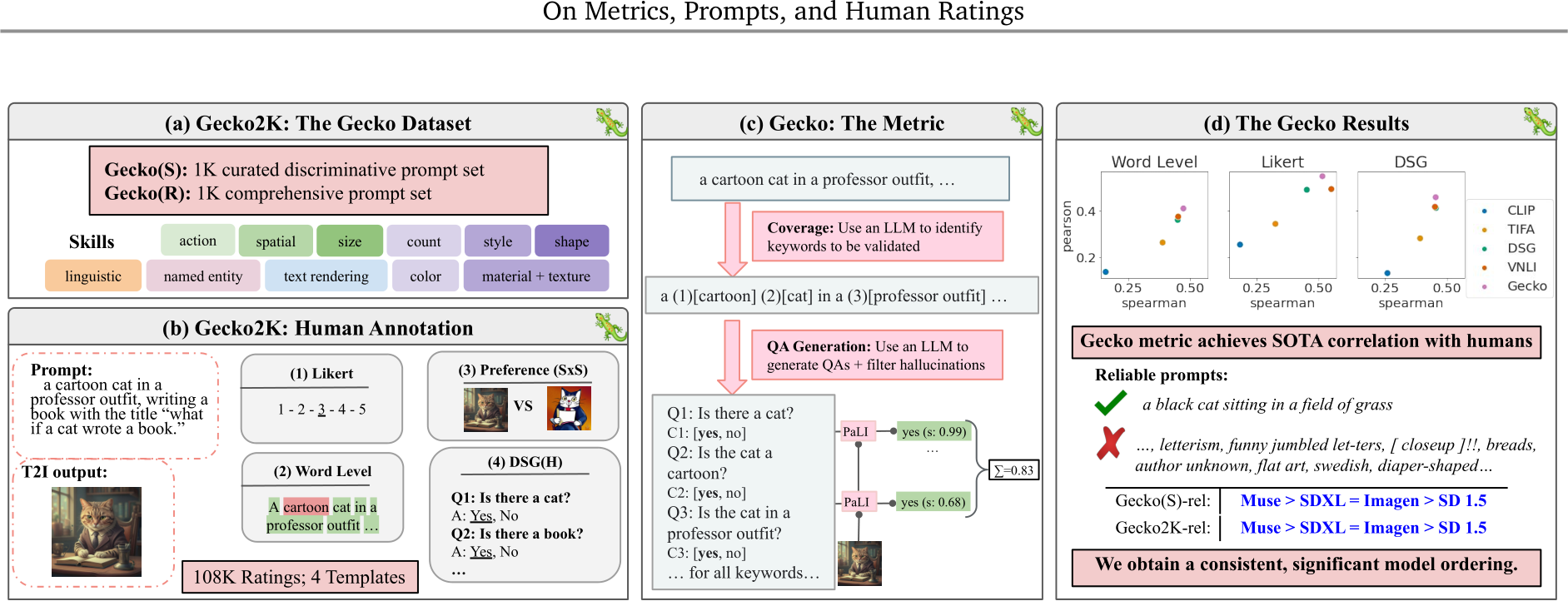
Figure 1 | The Gecko Framework. (a) Our Gecko2K dataset consists of two subsets covering a range of skills; Gecko(S) divides skills further into sub-skills. (b) In Gecko2K, we collect judgements for four human templates, resulting in 108K annotations. (c) The Gecko metric, which includes better coverage for questions, NLI filtering, and better score aggregation. (d) Experiments: using Gecko2K, we compare metrics, T2I models, and the human annotation templates.

For example, as visualised in Fig. 3, for text rendering, it probes if models can generate text of varying length, numerical values, etc.

Human judgement. Another key component is the human experiment design used to collect gold-standard data. One example is to ask the human raters to judge the image–text alignment on a fixed scale of 1 to 5. The design of human experiments, which we refer to as the annotation template, impacts the level of fine-grained information we can collect, i.e., whether a specific word is depicted or not. It might also affect the quality and reliability of the collected data. However, various work uses different annotation templates, making it hard to compare results across papers. As a result, we perform a comprehensive study of four main annotation templates (shown in panel (b) of Fig. 1) and collect ratings of four T2I models on Gecko2K. We observe that, across templates, SDXL [47] is best on Gecko(R) and Muse [7] is best on Gecko(S). We find that under Gecko(S), we are able to discriminate between models—all templates agree on a model ordering with statistical significance. For Gecko(R), while general trends are similar across templates, results are noisier. This demonstrates the impact of the prompt set when comparing models. Finally, we find some prompts (e.g., “stunning city 4k, hyper detailed photograph”) can be ambiguous, subjective, or hard to depict. As a result, we introduce a subset of reliable prompts where annotators agree across models and templates. Using this subset in Gecko(R), we observe a more consistent model ordering across templates, where the fine-grained annotation templates agree more.

Auto-eval metrics. Prior work comparing T2I automatic-evaluation (auto-eval) metrics [24, 49, 61, 29, 10] of alignment does so on small ground-truth datasets (with 2K raw annotations [29, 69]), where a handful of prompts are rated using one annotation template (see Table 1). Using our large set of human ratings (>100K), we thoroughly compare these metrics. We also improve upon the question-answering (QA) framework in [29] (panel (c) in Fig. 1). Our metric, Gecko, achieves state-of-the-art (SOTA) results when compared to human data as a result of three main improvements: (1) enforcing that each word in a sentence is covered by a question, (2) filtering hallucinated questions that a large language model (LLM) generates, and (3) improved VQA scoring.

Fig. 1 summarises our main contributions: (1) Gecko2K: A comprehensive and discriminative benchmark with a better coverage of skills and fine-grained sub-skills to identify failures in T2I models and auto-eval metrics. (2) A thorough analysis on the impact of annotation templates in model and

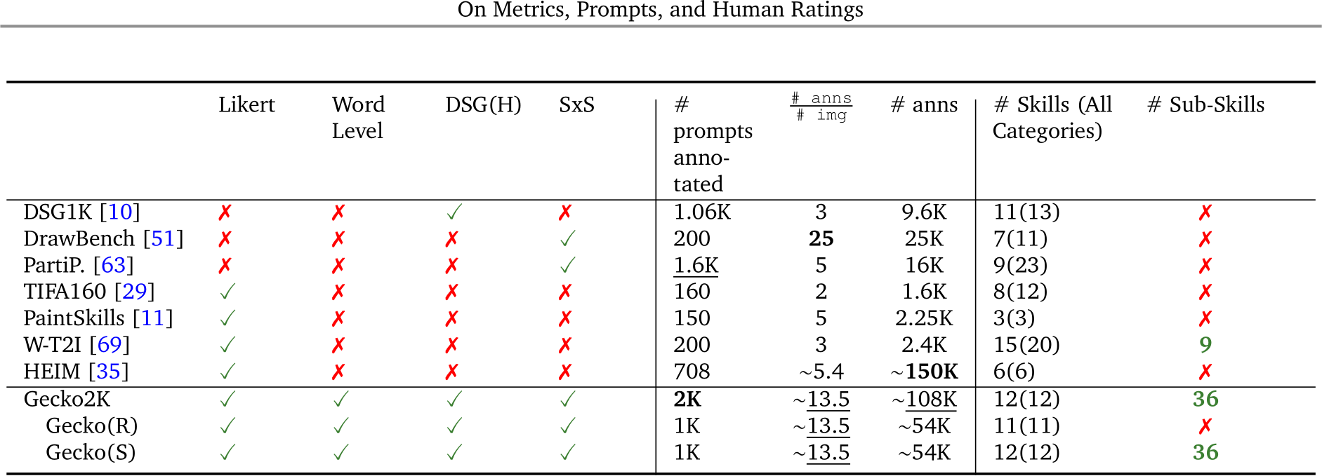
Table 1 | Comparison of annotated alignment datasets. We report the amount of human annotation and skill division for each dataset. We can see that many datasets include only a handful of annotated prompts or a small number of annotations (anns) per image or overall. No dataset besides Gecko2K collects ratings across multiple different human annotation templates. We also include the number of skills and sub-skills in each dataset. Again, Gecko includes the most number of sub-skills, allowing for a fine-grained evaluation of metrics and models. When datasets do not include skills, we map their categories into skills/sub-skills as appropriate.

metric comparisons, which leads us to introduce reliable prompts. (3) Gecko: An auto-eval metric that is SOTA across our challenging benchmark (Gecko(R)/(S) and the four annotation templates) and TIFA160 [29].

Benchmarking alignment in T2I models. Many different benchmarks have been proposed to holistically probe a broad range of model capabilities within T2I alignment. Early benchmarks are small scale and created alongside model development to perform side-by-side model comparisons [51, 63, 3]. Later work (e.g., TIFA [29], DSG1K [10] and HEIM [35]) focuses on creating holistic benchmarks by drawing from existing datasets (e.g., MSCOCO [40], Localized Narratives [48] and CountBench [45]) to evaluate a range of capabilities including counting, spatial relationships, and robustness. Other datasets focus on a specific challenge such as compositionality [30], contrastive reasoning [69], text rendering [57], reasoning [11] or spatial reasoning [19]. The Gecko2K benchmark is similar in spirit to TIFA and DSG1K in that it evaluates a set of skills. However, in addition to drawing from previous datasets—which may be biased or poorly representative of the challenges of a particular skill—we collate prompts across sub-skills for each skill to obtain a discriminative prompt set. Moreover, we gather human annotations across multiple templates and many prompts (see Table 1); as a result, we can reliably estimate image–text alignment and model performance.

Automatic metrics measuring T2I alignment. Image generation models initially compared a set of generations with a distribution from a validation set using Fréchet Inception Distance (FID) [25]. However, FID does not fully reflect human perception of image quality [54, 32] nor T2I alignment. Inspired by work in image captioning, a subsequent widely used auto-eval metric for T2I alignment is CLIPScore[24]. However, such metrics poorly capture finer-grained aspects of image–text understanding, such as complex syntax or objects [5, 64]. Motivated by work in natural language processing on evaluating the factuality of summaries using entailment or QA metrics [43, 34, 28], similar metrics have been devised for T2I alignment. VNLI [61] is an entailment metric which finetunes a pretrained vision-and-language (VLM) model [8] on a large dataset of image and text pairs. However, such a metric may not generalise to new settings and is not interpretable—one cannot diagnose why an

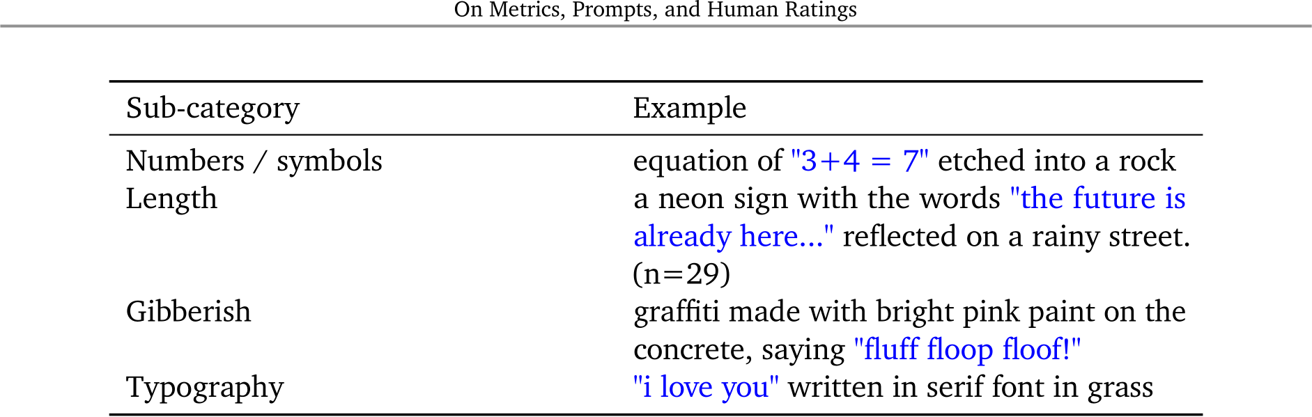
Table 2 | Subcategories and corresponding motivations for the text rendering skill.

alignment score is given. Visual question answering (VQA) methods such as TIFA [29], VQ2 [61] and DSG [10] do not require task-specific finetuning and give an interpretable explanation for their score. These metrics create QA pairs which are then scored with a VLM given an image and aggregated into a single score. However, the performance of such methods is conditional on the behaviour of the underlying LLMs used for question generation, and VLMs used for answering questions. For example, LLMs might generate questions about entities that are not present in the prompt or may not cover all parts of the prompt. By enforcing that the LLM does indeed cover each keyword in the prompt and by filtering out hallucinated questions, we are able to substantially improve performance over other VQA-based metrics.

We curate a fine-grained skill-based benchmark with good coverage. If we do not have good coverage and include many prompts for one skill but very few for another, we would fail to highlight a model or a metric’s true abilities. We also consider the notion of sub-skills—for a given skill (e.g., counting), we curate a list of sub-skills (e.g., simple modifier: ‘1 cat’ vs additive: ‘1 cat and 3 dogs’). This notion of sub-skills is important as, without it, we may be testing a small, easy part of the distribution such as generating counts of 1-4 objects and not the full distribution that we care about. We introduce two new prompt sets within Gecko2K: Gecko(R) and Gecko(S). Gecko(R) extends the DSG1K [10] benchmark by using automatic tagging to improve the distribution of skills (see App. C for details). However, it does not consider sub-skills nor cover the full set of skills we are interested in. Moreover, a given prompt (as in DSG1K and similar datasets) may evaluate for many skills, making it difficult to diagnose if a specific skill is challenging or if generating multiple skills is the difficult aspect. As a result, we also introduce Gecko(S), a curated skill-based dataset with sub-skills. Finally, we gather a large number of annotations per image across four templates (see Table 1) but defer to Sec. 4 for details.

3.1. Gecko(R): Resampling Davidsonian Scene Graph Benchmark

The recent Davidsonian Scene Graph Benchmark (DSG1K, [10]) curates a list of prompts from existing datasets∗ but does not control for the coverage or the complexity degrees of a given skill. The authors randomly sample 100 prompts and limit the prompt length to 200 characters.

The resulting dataset is imbalanced in terms of the distribution of skills. Also, as T2I models take in longer and longer prompts, the dataset will not test models on that capability. We take a principled approach in creating Gecko(R) by resampling from the base datasets in DSG1K for better coverage

∗TIFA[29], Stanford Paragraphs [33], Localized Narratives [48], CountBench [45], VRD [42], DiffusionDB [59], Midjourney [58], PoseScript [14], Whoops [4], DrawText-Creative [41].

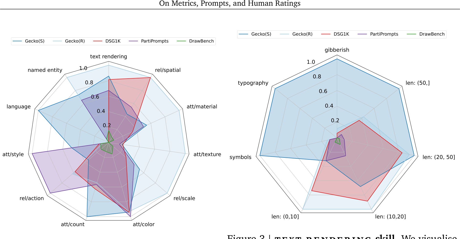
Figure 2 | Distribution of skills. We visualise the distribution of prompts across different skills for Gecko(S)/(R), DSG1K [10], PartiPrompts [63] and DrawBench [51]. We use automatic tagging and, for each skill, normalise by the maximum number of prompts in that skill over all datasets. For most skills, Gecko2K has the most number of prompts within that skill.

Figure 3 | text rendering skill. We visualise the distribution of prompts across seven sub-skills explained in Table 2 (‘len: ...’ corresponds to bucketing different lengths of the text to be rendered). We normalise by the maximum number of prompts in the sub-skill (note that we only count unique texts to be rendered). The Gecko(S) dataset fills in much more of the distribution here than other datasets.

and lifting the length limit. After this process, there are 175 prompts longer than 200 characters and a maximum length of 570 characters. Also, this new dataset has better coverage over a variety of skills than the original DSG1K dataset (see Fig. 2).

While resampling improves the distribution of skills, it has the following shortcomings. Due to the limitations of automatic tagging, it does not include all skills we wish to explore (e.g., language). It also does not include sub-skills: most text rendering prompts do not focus on numerical text, non-English phrases (e.g., Gibberish), the typography, or longer text (see Fig. 3). Finally, automatic tagging can be error prone.

3.2. Gecko(S): A Controlled and Diagnostic Prompt Set

The aim of Gecko(S) is to generate prompts in a controllable manner for skills that are not well represented in previous work. We divide skills into sub-skills to diversify the difficulty and content of prompts. We take inspiration from psychology literature where possible (e.g., colour perception) and known limitations of current text-to-image models to devise these sub-skills. We first explain how we curate these prompts before discussing the final set of skills and sub-skills.

Curating a controlled set of prompts with an LLM. To generate a set of prompts semi-automatically, we use an LLM. We first decide on the sub-skills we wish to test for. For example, for text rendering, we may want to test for (1) English vs Gibberish to evaluate the model’s ability to generate uncommon words, and (2) the length of the text to be generated. We then create a template which conditions the generation on these properties. Note that as we can generate as much data as desired, we can define a distribution over the properties and control the number of examples generated for each sub-skill. Finally, we run the LLM and manually validate that the prompts are reasonable, fluent, and match

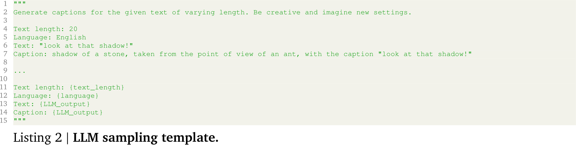
the conditioning variables (e.g., the prompt has the right length and is Gibberish / English). A sample template is given in App. C.3.

Gecko(S) make up. Using this approach and also some manual curation, we focus on twelve skills falling into five categories (Fig. 7): (1) named entities; (2) text rendering; (3) language/linguistic complexity; (4) relational: action, spatial, scale; (5) attributes: color, count, surfaces (texture/material), shape, style. An overview is given in Fig. 7. We give more details here about how we break down a given skill, text rendering, into sub-skills but note that we do the same for all categories; details are in App. G. For text rendering, we consider the sub-skills given in Table 2. Using this approach, we get better coverage over the given sub-skills than other datasets (including Gecko(R)) as shown in Fig. 3 and we find results are consistent across different annotation templates.

When evaluating T2I models, existing work uses different annotation templates for collecting human judgements. While human annotation is the gold-standard for evaluating generative models, previous work shows the design of a template and background of annotators can significantly impact the results [12]. For example, a common approach is to use a Likert scale [39] where annotators evaluate the goodness of an image with a fixed scale of discrete ratings. However, previous work [10, 29, 35] uses different designs (e.g., scales from 1 to 5 vs 1 to 3), so results cannot be directly compared. We examine differences between templates and how the choice of a template [10, 38] impacts the outcomes when comparing four models: SD1.5 [50], SDXL [46], Muse [7], and Imagen [51]. (Imagen and Muse are variants based on the original models, but trained on internal data sources.) We consider three absolute comparison templates (Likert, Word Level, and DSG(H)) which evaluate models individually, and a template for relative comparison (SxS). The templates are defined below and a high-level visualisation of each template is in panel (b) of Fig. 1. More details are in App. E.1.

4.1. Annotation Templates

Likert scale. We follow the template of [10] and collect human judgements using a 5-point Likert scale by asking the annotators “How consistent is the image with the prompt?” where consistency is defined as how well the image matches the text description. Annotators are asked to choose a rating from the given scale, where 1 represents inconsistent and 5 consistent, or a sixth Unsure option for cases where the text prompt is not clear. Choosing this template enables us to compare our results with previous work, but does not provide fine-grained, word-level alignment information. Moreover, while Likert provides a simple and fast way to collect data, challenges such as defining each rating especially when used without textual description (e.g., what 2 refers to in terms of image–text consistency), can lead to subjective and biased scores [23, 37].

Word-level alignment (WL). To collect word-level alignment annotations, we use the template of [38] and define an overall image–text alignment score using the word-level information. Given a text–image pair, raters are asked to annotate each word in the prompt as Aligned, Unsure, or Not aligned. Note that for each text–image pair under the evaluation, the number of effective annotations a rater must perform is equal to the number of words in the text prompt. Although potentially more time consuming than the Likert template,† We compute a score for each prompt–image pair per rater by aggregating the annotations given to each word. A final score is then obtained by averaging the scores of 3 raters. More details can be found in App. E.1.

DSG(H). We also use the annotation template of [10] that asks the raters to answer a series of questions for a given image, where the questions are generated automatically for the given text prompt as discussed in [10].

In addition, raters can mark a question as Invalid in case a question contradicts another one. The total number of Invalid ratings per evaluated generative model is given in App. E.1. Annotators could also rate a question as Unsure, in cases where they do not know the answer or find the question subjective or not answerable based on the given information.

For a given prompt, the number of annotations a rater must complete is given by the number of questions. We calculate an overall score for an image–prompt pair by aggregating the answers across all questions, and then averaging this number across raters to obtain the final score.

Side-by-side (SxS). We consider a template in which pairs of images are directly compared. The annotators see two images from two models side-by-side and are asked to choose the image that is better aligned with the prompt or select Unsure. We obtain a score for each comparison by computing the majority voting across all 3 ratings. In case there is a tie, we assign Unsure to the final score of an image–prompt pair.

Data Collection Details. We recruited participants (N = 40) through a crowd-sourcing pool. The full details of our study design, including compensation rates, were reviewed by our institution’s independent ethical review committee. All participants provided informed consent prior to completing tasks and were reimbursed for their time. Considering all four templates, both Gecko subsets, and the four evaluated generative models, approximately 108K answers were collected, totalling 2675 hours of evaluation.

4.2. Comparing Annotation Templates

We first evaluate the reliability of each absolute comparison template by measuring inter-annotator agreement—does the choice of the template impact the quality of the data we can collect?

We compute Krippendorff’s ] for each generative model and template and report the results in Table 3. Krippendorff’s assumes values between -1 and 1, with 1 indicating perfect agreement and 0 chance level [65]. As our goal is evaluating agreement between annotators, in this experiment we keep all Unsure ratings, but for the following experiments we pre-process the annotations by removing all such ratings so as to only reflect cases where annotators were confident. We observe that all the templates yield agreement above chance levels for all generative models, with 5, except for the Likert–SD1.5 pair for Gecko(R). We also observe that for Gecko(R), WL is a more reliable template but for synthetic prompts, DSG(H) has higher agreement We then investigate which templates agree/disagree more with each other by computing Spearman’s rank and Pearson correlations between scores from each template. Results are in App. E.2 and show that there is an overall high correlation between all templates on both Gecko(S)/(R) and the strongest observed correlation among all models and metrics is between the finer-grained templates, WL and DSG(H), on Gecko(S).

Reliable Prompts. Given the human ratings we have collected, we can examine how reliable a prompt is—the extent to which the annotators agree in their ratings regardless of the annotation template and the model used to generate images. To get a set of reliable prompts, for each model– template pair, we select the prompts for which inter-rater disagreement‡ is below 50% the maximum disagreement observed across all prompts for that model–template pair. We then repeat this step

‡Defined as the variance across the scores given by each rater in the case of Likert, and the average variance across words and questions scores in the case of WL and DSG(H), respectively.

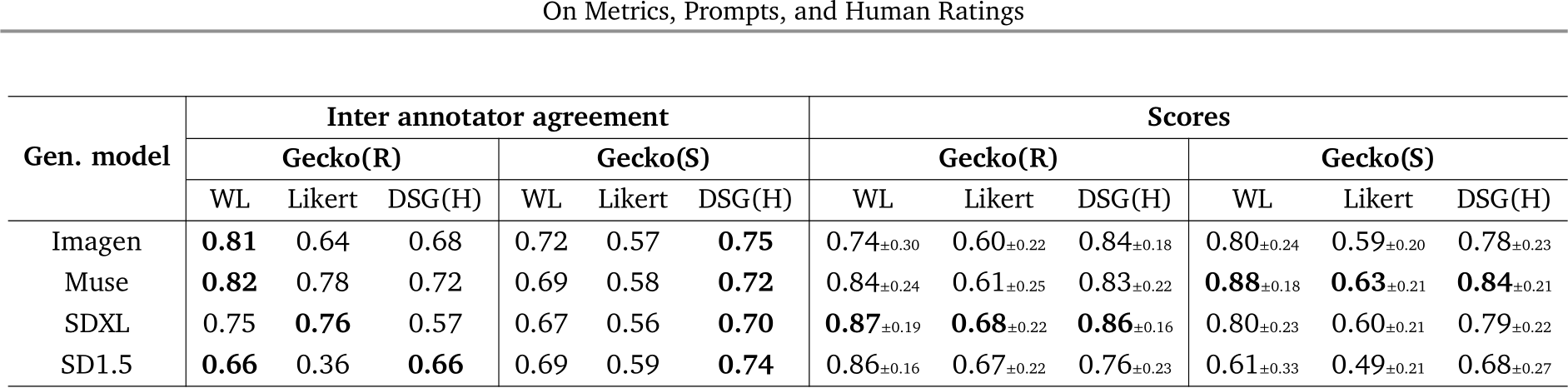
Table 3 | Inter-annotator agreement and ratings for all models and templates. We measure inter-annotator agreement for each human evaluation template with Krippendorff’s . Higher values indicate better agreement. We also show the mean and standard deviation for the scores of all templates after mapping the ratings to the [0, 1] interval, with 1 indicating perfect alignment.

for all model–template pairs, and consider the intersection of prompts across these settings as the reliable prompts. We further refine this set by removing instances for which all ratings from the Likert template are Unsure. This procedure yields a total of 531 and 725 reliable prompts for Gecko(R) and Gecko(S), respectively. As we only consider ratings from the absolute comparison templates when finding reliable prompts, we investigate how the SxS template agreement (i.e., Krippendorff’s ) changes given this set. This experiment validates our notion of reliability by evaluating if it is transferable to other templates. For Gecko(R), we find that using reliable prompts increases the average Krippendorff’s from 0.45 to 0.47, and for Gecko(S) from 0.49 to 0.54, showing that both sets of reliable prompts generalise to other templates. Detailed results are in App. E.2.

SxS comparison. To compare the SxS template with the absolute comparison ones, we compute the accuracy obtained by each absolute template when predicting the preferred model given by SxS annotations with the reliable subsets of both Gecko(R) and Gecko(S). For Gecko(R), we find that DSG(H) presented the best accuracy in 4 out of 6 evaluations, followed by Likert which was the most accurate absolute template in the remaining 2 evaluations. On the other hand, for Gecko(S), we find that WL and Likert predict SxS judgements with higher accuracy, each one being the most accurate template in 3 out of 6 cases, indicating that, overall, Likert scores were able to better predict results of SxS comparisons. The complete set of results is in App. E.2.

4.3. Comparing I2T Models

We first compare the T2I models with the human ratings collected using the three absolute comparison templates as they presented overall higher inter annotator agreement. In Table 3, we report the average and standard deviation of all ratings. We verify the significance of outcomes by performing the Wilcoxon signed-rank test for all pairs of models with 001. Where results indicate the null-hypothesis is rejected (i.e., the distribution of ratings is significantly different), we can say there is enough evidence that one model is better than another. To determine which model is best, we compare the mean values of their scores. Fig. 4 presents the results for the comparisons between all pairs of models with reliable (Gecko(*)-rel) prompt subsets. When considering significance in Fig. 4, we see that Muse is not worse than any of the contenders across all templates and prompt sets; we determine it is the best overall model given human judgement. Also, SD1.5 is worse or the same as other models except for Imagen when evaluated with Gecko(R)-rel.

Fig. 4 results also shed light on the agreement between templates: for Gecko(S)-rel all templates agree with each other, and for Gecko2K-rel all templates agree or do not contradict each other (i.e., one is significant, the other not).

Summary. We see that our discriminative prompt set, Gecko(S), results in consistent model rankings,

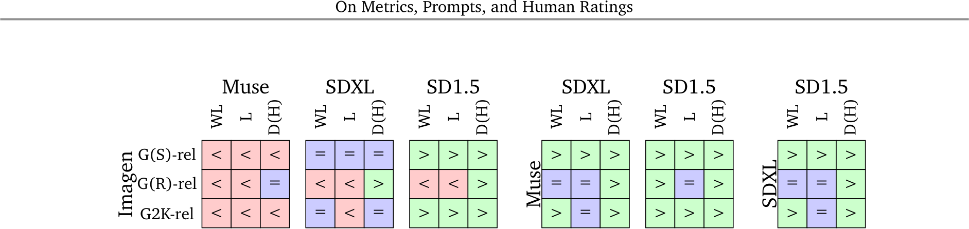
Figure 4 | Comparing models using human annotations. We compare model rankings on the reliable subsets of Gecko(S) (G(S)-rel), Gecko(R) (G(R)-rel) and both subsets (G2K-rel). Each grid represents a comparison between two models. Entries in the grid depict results for WL, Likert (L), and DSG(H) (D(H)) scores. The > sign indicates the left-side model is better, worse (<), or not significantly different (=) than the model on the top.

independent of the template used. For prompts that test for aspects other than image–text alignment, i.e., Gecko(R), the choice of the annotation template impacts the ordering of the models, but the best and worst models are mostly consistent across templates. In terms of templates, the finer-grained ones (WL and DSG(H)) have better inter-annotator agreement in comparison to Likert and SxS. We also notice that when comparing model rankings with Gecko(R)-rel, DSG(H) is the template that mostly disagrees with the others. This finding, along with the higher inter-annotator agreement shown by the WL template, makes it the overall best choice for evaluating image–text alignment on Gecko2K.

Question answering (QA) based metrics have the advantage of attributing failures to specific questions as opposed to giving a single, uninterpretable score (as in VNLI [61] and CLIP [49]), and benefit from the increasing capabilities of LLMs and VQA models. The Gecko metric improves upon QA [29, 10, 61] metrics by enforcing coverage of the prompt and reducing hallucinations. A standard QA setup (from [29]) consists of three steps: (1) QA generation: prompting an LLM to generate a set of binary question-answer pairs 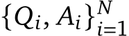on a given T2I text description . (2) VQA assessment: employing a VQA model to predict answer for the generated questions given the generated image . (3) Scoring: computing the alignment score by assessing the VQA accuracy using Eq. (1).

However, this pipeline exhibits several limitations. First, controlling the quantity of QA pairs generated, especially from lengthy sentences, poses a challenge. In such cases, the prompted LLM often selectively generates questions for specific segments of the text while overlooking others. Second, LLMs are prone to producing hallucinations [2, 20], leading to the generation of low-quality, unreliable QA pairs. Furthermore, the reliance on binary judgement—strictly matching without considering the predicted probability of —overlooks the inherent uncertainty in the predictions.

While TIFA[29] and DSG[10] have proposed some solutions to overcome some of the limitations highlighted above, such as using a QA model to verify the generated QAs or breaking the prompt into atomic parts, the effectiveness of these solutions remains limited, especially on more complicated text prompts. Here we propose a simpler, but more robust method that consistently outperforms on various benchmarks.

Coverage. To improve the coverage of questions over the text sentence , we split the QA generation

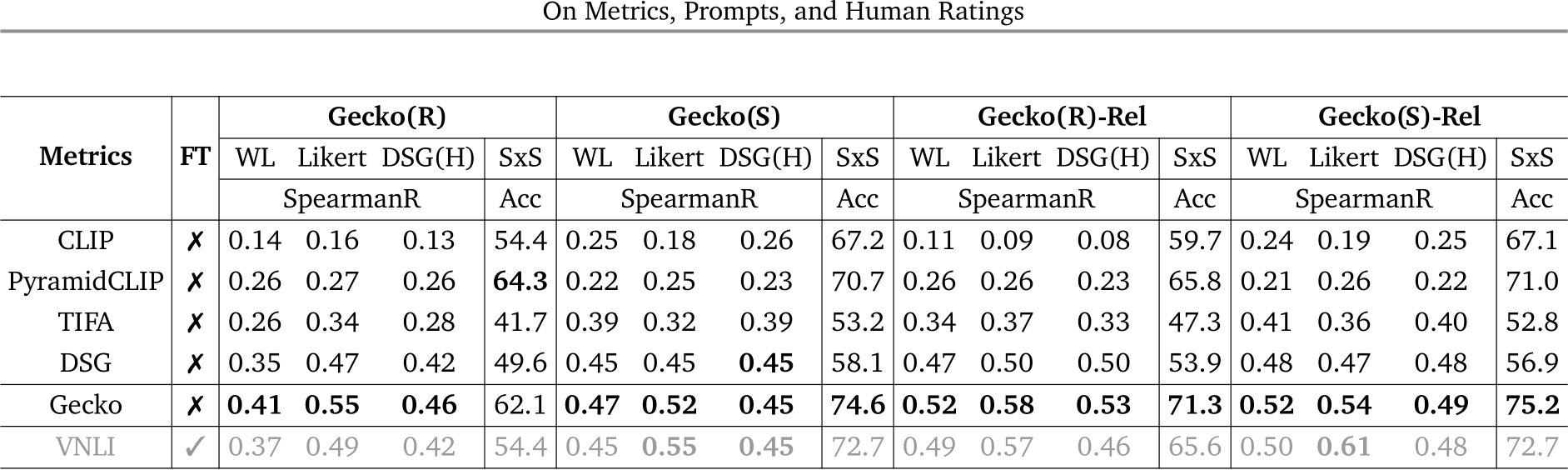
Table 4 | Correlation between VQA-based, contrastive, and fine-tuned (FT) auto-eval metrics and human ratings across annotation templates on Gecko2K and Gecko2K-Rel. Gecko scores highest in 13/14 conditions, even out-performing the fine-tuned VNLI metric.

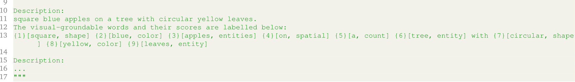
into two distinct steps. We first prompt the LLM to index the visually groundable words in the sentence. For example, the sentence ‘A red colored dog.’ is transformed into ‘A {1}[red colored] {2}[dog].’ Subsequently, using the text with annotated keywords as input, we prompt the LLM again to generate a QA pair for each word labelled in an iterative manner (see App. D for the prompting details). This two-step process ensures a more comprehensive and controllable QA generation process, particularly for complex or detailed text descriptions.

NLI filtering. For filtering out the hallucinated QA pairs, inspired by previous work in NLP [43, 34], we employ an Natural Language Inference (NLI) model [27] model for measuring the factual consistency between the text and QA pairs . QA pairs with a consistency score lower than a pre-defined threshold are removed, ensuring that only the factually aligned ones are retained.

VQA score normalisation. The final improvement we make is how to aggregate scores from the VQA model. The motivation is that the VQA model can predict a very similar score for two answers. If we simply take the max, then we lose this notion of uncertainty reflected in the scores of the model. If the negative log likelihood of answer and the correct answer is , we normalise the scores as follows:

To compare auto-eval metrics, we perform two sets of experiments: first, we compare how various metrics correlate with human judgements—whether their predicted alignment scores match those of the raters for each prompt. We demonstrate that the proposed Gecko metric consistently performs best in Sec. 6.2 for Gecko(S)/(R) and analyse results per category for Gecko(S). Additionally, we validate the utility of each component.

Finally, in Sec. 6.3, we validate that metrics give the same model ordering as human judgements and find that Gecko is the same or better than other metrics at this task.

6.1. Experimental Setup

Metrics Evaluated. We benchmark three types of auto-eval metrics on Gecko2K: (1) contrastive models: CLIP[49] and PyramidCLIP [16]; (2) NLI models: VNLI [61]; (3) QA-based methods: TIFA [29], DSG [10] and our proposed metric Gecko.

Pre-trained Models. We use a ViT-B/32 [15] model for CLIP and ViT-B/16 [15] for PyramidCLIP

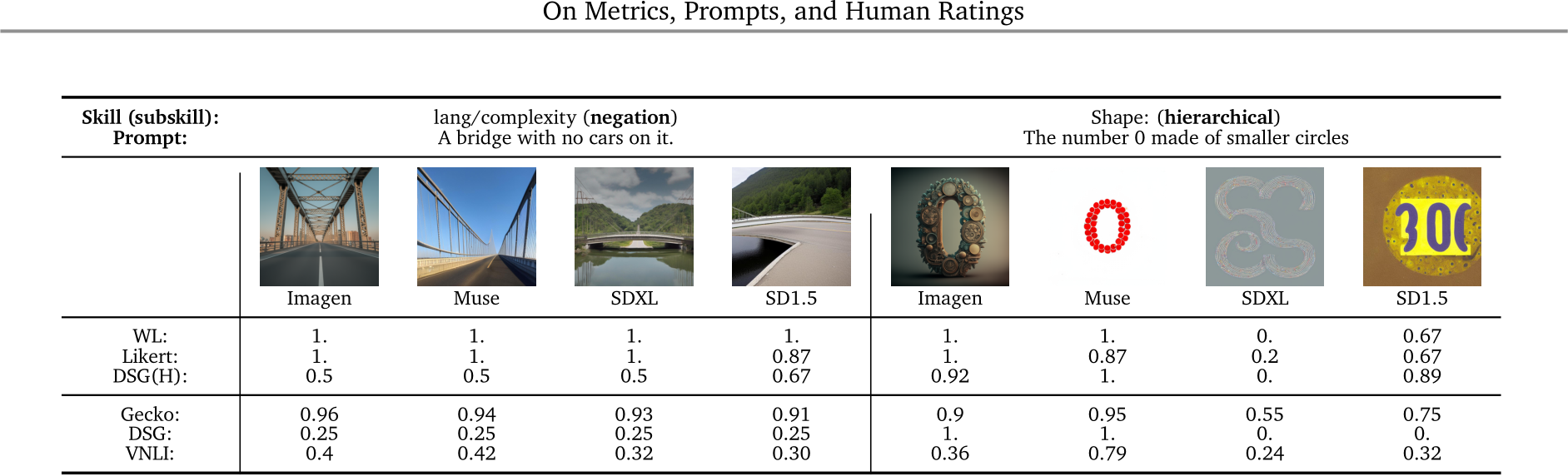
Figure 6 | Visualisations of scores from different auto-eval metrics. We show the image generations by the four generative models given two prompts from Gecko(S), with the alignment scores estimated by human annotators and auto-eval metrics.

in our experiments. For all the VQA-based models, we use PaLM-2 [1] as the LLM and PaLI [8] as the VQA model for fair comparison. When evaluating the Gecko metric, we use a T5-11B NLI model from [27] and set the threshold at 0.005. This threshold was determined by examining QA pairs with NLI probability scores below 0.05. We observed that QAs with scores below 0.005 are typically hallucinations. We re-use the original prompts from TIFA for generating QAs, and add coverage notation to their selected texts as described in Sec. 5.

Finally, some baseline models are trained with a maximum text input length and 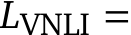82, thus unable to process longer descriptions; for these models, we only take the first tokens from the texts as input.

6.2. Correlation with Human Judgement

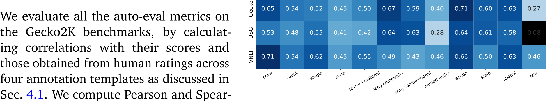
Figure 5 | Per skill results of Gecko, DSG and VNLI. We visualise the Likert correlation for each skill. Where p-values are > 0.05, we colour the square black. Results

Results on Gecko(R). We first compare the auto-eval metrics (CLIP, TIFA, DSG, Gecko) that do not rely on fine-tuning (results and findings from additional auto-eval metrics are in Sec. G.3.) As shown in Tab. 4, the Gecko metric outperforms the others and shows a higher correlation with most of the human annotation templates. As expected, contrastive metrics (CLIP variants) are worse overall than QA-based metrics, as they only measure coarse-grained alignment at the sentence level. However, it is worth noting that a better CLIP model (e.g., PyramidCLIP) can be a very strong baseline on SxS accuracy, showing its superior ability in doing pair-wise comparison.

DSG is the second best metric, except on SxS where it ranks third. It outperforms TIFA by a clear margin but falls behind Gecko. Finally, we compare Gecko with VNLI, our supervised baseline as the VNLI model is fine-tuned for text–image alignment on a mixed dataset containing COCO (which is used in DSG(R)), while other metrics are not fine-tuned. Nonetheless, Gecko still shows a much

Table 5 | Ablation on proposed Gecko metric on Gecko2K. We ablate the effectiveness of the three proposed improvements by adding them to the TIFA baseline one by one. They all bring higher correlation with human judgement across the board on Gecko2K.

higher correlation with WL, Likert and DSG(H).

Results on Gecko(S). As shown in Tab. 4, we observe a similar pattern to Gecko(R) on our synthetic subset, Gecko(S): the Gecko metric has the highest correlation with human ratings; DSG is the second best metric, except for the SxS template where CLIP outperforms it. Given a template, the correlation scores are generally higher on Gecko(S) which is not surprising at this benchmark focuses on measuring alignment. To better understand the differences between auto-eval metrics/annotation templates with respect to various skills, we visualise a breakdown of skills in Gecko(S) in Fig. 5 and App. F.1,G.4. Different metrics have different strengths: for example, we see that while Gecko and VNLI metrics are consistently good across skills, the Gecko metric is better on more complex language, DSG is better on compositional prompts, and VNLI is better on text rendering. We visualise examples in Fig. 6. For the negation example, we can see that VNLI and DSG mistakenly think none of the images are aligned. We can also see that the reason DSG(H) gives inconsistent results with WL/Likert here is that the question generation is confused by the negation (asking if there are cars as opposed to no cars). VNLI and DSG perform better on the shape prompt but VNLI scores Imagen incorrectly and DSG gives hard results (0 or 1) and so is not able to capture subtler differences in the human ratings.

Results on Gecko2K-Rel. We also include the correlation of metrics on reliable prompts in Tab. 4. We can see that on this reliable subset, the Gecko metric shows even better results by outperforming other metrics on everything. Furthermore, we observe that when moving from Gecko2K to Gecko2K-Rel, all the correlation scores between the QA-based metrics and human ratings increase, while those of the CLIP variants drop. This shows that the relatively high correlations from CLIP in the full-set has some noise, and QA-based metrics align more closely with human judgement.

Ablation on proposed Gecko metric. We ablate the impact of the three key improvements we propose, namely, QA generation with coverage, linear normalisation of predicted probabilities, and NLI filtering on QA. Starting from our baseline TIFA, we include the improvements one at a time to see the benefits brought. The results in Tab. 5 uniformly demonstrate a positive impact from each improvement. Notably, NLI filtering brings the largest boost among the three, underscoring the limitation of LLMs in reliably generating high-quality and accurate QA pairs.

Results on TIFA160. We compare the Gecko metric with other metrics on TIFA160 [29]. It is a set of 160 text–image pairs, each with two Likert ratings. In Tab. 6, we list the results of other metrics reported in [29, 10], and compare them with Gecko as well as our re-implementation of TIFA and DSG. Gecko has the highest correlation with Likert scores, with an average correlation 0.07 higher than that of DSG, when using the same QA and VQA models. This shows that the power of our proposed metric is from the method itself, not from the advance of models used.

6.3. Model-ordering Evaluation

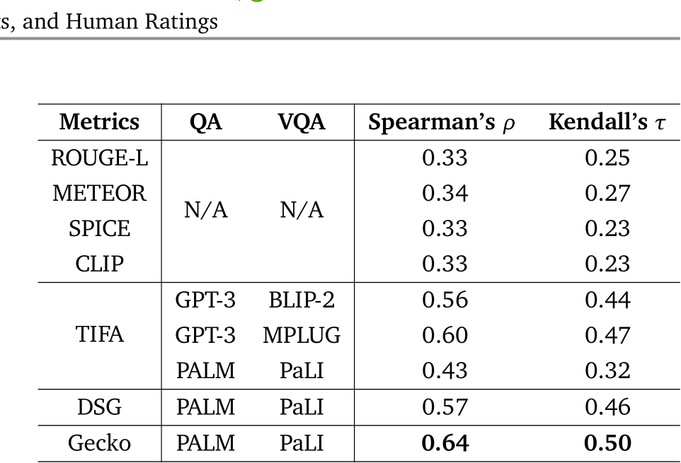
Table 6 | Comparing different metrics by their correlation with human Likert ratings on TIFA160. The Gecko metric outperforms the oth-

We next examine if each auto-eval metric can predict how two models are ordered according to the human ratings. We use the results obtained by comparing T2I models with scores from all absolute comparison templates reported in Fig. 4 and consider the majority relation assigned to a model pair as the ground truth: if two of the templates find model 1 is better than model 2, then we assume model 1 > model 2. Given the ground-truth relation between a model pair, we then count the number of times an auto-eval metric successfully found the same relation, in terms of both significance and direction. In addition, we count the number of times an auto-eval metric captured the ground-truth relationship following

the most common practice in the literature: ordering models by solely comparing the mean values of scores regardless of statistical significance. In App. G.2, we show the results for all auto-eval metrics on both Gecko(R) and Gecko(S). Our results highlight that the number of significant successful comparisons is lower than comparisons with mean values. All metrics except for DSG and CLIP get the same number of successful comparisons for both criteria. Note that Gecko not only is within the metrics that best capture pairwise model orderings as per the human eval ground-truth values, but Gecko scores are also the best correlated with the human scores themselves (as we can see in Table 4).

We took stock of auto-eval of T2I models and the three main components: the benchmark, the annotation templates, and the auto-eval metric. We introduced the Gecko2K benchmark, gathered ratings across four templates and introduced a notion of reliable prompts; we also developed Gecko—a SOTA VQA auto-eval metric. We conclude the following takeaways: (1) Fine-grained annotation templates (e.g., WL, DSG(H)) are more consistent with each other than coarse-grained (e.g., Likert and SxS) and vice versa. (2) If using reliable prompts and templates with high inter-annotator agreement, we get a consistent model ordering (irrespective of the choice of prompts—e.g., Gecko(R)/(S)). (3) When comparing auto-eval metrics, it is better to use ‘reliable’ prompts, as they better measure alignment, give better signal from raters and a more consistent ordering of metrics and models.

Our work highlights the importance of standardising the evaluation of models with respect to both the benchmark used and also the annotation template. While our proposed metric can be reliably used for model comparisons, it is still limited by the quality of the pre-trained LLMs and VLMs in the pipeline. Consequently, an interesting future direction is to provide a confidence threshold in addition to the metric scores.

Acknowledgements We thank Nelly Papalampidi, Zi Wang, Miloš Stanojević, and Jason Baldridge for their feedback throughout the project. We are grateful to Nelly Papalampidi and Andrew Zisserman for their feedback on the manuscript. We thank Aayush Upadhyay and the rest of the Podium team for their help in running models.

A Appendices 14

B Overview 15

C Gecko2K: More details 15

C.1 Automatic tagging for Gecko(R) . . . . . . . . . . . . . . . . . . . . . . . . . . . . . . 15

C.2 Prompt distribution in Gecko(R) . . . . . . . . . . . . . . . . . . . . . . . . . . . . . . 16

C.4 Breakdown by skill/sub-skill in Gecko(S) . . . . . . . . . . . . . . . . . . . . . . . . . 17

D Gecko Metric: More details 22

D.1 LLM prompting for generating coverage . . . . . . . . . . . . . . . . . . . . . . . . . 22

D.2 LLM prompting for generating QAs . . . . . . . . . . . . . . . . . . . . . . . . . . . . 22

E Human annotation: more details and experiments 24

E.1 Annotation templates . . . . . . . . . . . . . . . . . . . . . . . . . . . . . . . . . . . . 24

E.2 Additional experimental results . . . . . . . . . . . . . . . . . . . . . . . . . . . . . . 26

E.3 Reliable prompts: Examples of image-prompt pairs with high human (dis)agreement 27

E.4 Human evaluation templates: Challenging cases . . . . . . . . . . . . . . . . . . . . . 33

F T2I Models: Additional comparisons 35

F.1 Analysing Model Ratings Per Skill . . . . . . . . . . . . . . . . . . . . . . . . . . . . . 35

F.2 Model comparisons with TIFA160 . . . . . . . . . . . . . . . . . . . . . . . . . . . . . 38

G Auto-eval metrics: Additional experiments 38

G.1 Pearson correlation Gecko2K. . . . . . . . . . . . . . . . . . . . . . . . . . . . . . . . 38

G.2 Model-ordering Evaluation . . . . . . . . . . . . . . . . . . . . . . . . . . . . . . . . . 39

G.3 Results for Additional Metrics on the Gecko Benchmark . . . . . . . . . . . . . . . . . 39

G.4 Analysing Auto-Eval Metric results per skill. . . . . . . . . . . . . . . . . . . . . . . . 40

G.5 Additional visualisations. . . . . . . . . . . . . . . . . . . . . . . . . . . . . . . . . . . 40

G.6 Results per Word for WL . . . . . . . . . . . . . . . . . . . . . . . . . . . . . . . . . . 40

In the Appendix, we give additional information on the benchmark, human annotation and corresponding results for T2I models, and experimental results for the auto-eval metrics.

Gecko Benchmark: For the benchmark, we give further information on how we automatically tag Gecko(R) and semi-automatically generate prompts in Gecko(S) in Appendix C.1 and C.3 respectively. We then give more detail about the skill breakdown in Gecko(R) in App. C.2. We define and give examples for the sub-skills in Gecko(S) in App. C.4.

Human Annotation: For the human annotation, we give additional details of our setup including screenshots of the annotation templates used and qualitative limitations of each setup in App. E.1. We further discuss more experimental results comparing inter-annotator agreement and the raw predictions under each template in App. E.2. Finally, we visualise the most and least reliable prompts in App. E.3, giving an intuition for the properties of the prompt that lead to more or less agreement across templates.

Additional results on T2I models: We give further results on using the annotated data to (1) compare T2I models by skill in App. F.1. We also compare how well prompts in TIFA160 are able to discriminate models under our human annotation setup in App. F.2.

Additional results for auto-eval metrics: Finally, we give additional results for the auto-eval metrics, including more correlation results in App. G.1, the raw results for the model-ordering evaluation in App. G.2 and results for different CLIP variants in App. G.3. We then explore results per skill for different auto-eval metrics in App. G.4, give additional visualisations in App. G.5 and demonstrate that we can use Gecko to evaluate the per-word accuracy of the metric (this is not possible with other auto-eval metrics) in App. G.6.

As described in Sec. 3.1, we use automatic tagging in order to tag prompts with different skills in Gecko(R). However, this has a few issues: (1) it can be error prone; (2) we are limited by the tagging mechanism in the skills that we tag; (3) we do not tag sub–skills. As a result, we devise a semi-automatic approach to build Gecko(S) by few-shot prompting an LLM, as discussed in Sec. 3.2 and curate a dataset with a number of skills and sub-skills for each skill.

C.1. Automatic tagging for Gecko(R)

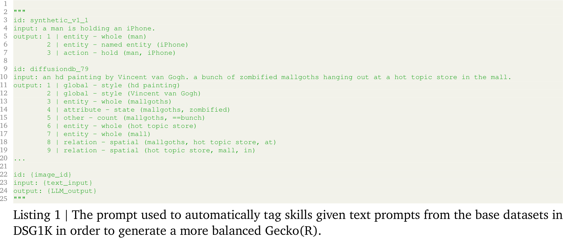
As mentioned in Sec. 3.1, to obtain a better control for the skill coverage and prompt length, we resampled from the 10 datasets used in DSG1k[10]. To identify the categories covered in the prompts, we adopted an automatic tagging method similar to that used in DSG1K. This method utilizes a Language Model (LLM) to tag words in the text prompt, as shown in Listing 1. The only difference is that we also included named entities and landmarks to be the original categories, such as whole, part, state, color etc.

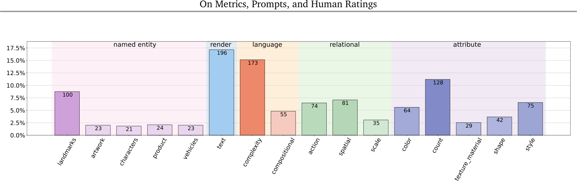
Figure 7 | Overview of Gecko(S). The set of skills (coloured by the corresponding category) covered by the synthetic prompts. Note that we gather prompts by breaking each skill into sub-kills.

C.2. Prompt distribution in Gecko(R)

We resample 1000 prompts from the base datasets used in DSG1K and ensure a more uniform distribution over skills and prompt length. To sample more prompts featuring words from under-represented skills (e.g.text rendering, shape, named identity and landmarks), we use automatic tagging in Appendix C.1 to categorize the words in all prompts as pertaining to a given skill. We then resample, assigning higher weights to the under-represented skills. The resulting skill distribution is shown in Fig. 8. Although the resampling increases the proportion of under-represented skills, the overall distribution remains unbalanced. This underscores the necessity of acquiring a synthetic subset with a more controlled and balanced prompt distribution. To sample long prompts, we eliminate the constraint set in DSG1K[10], which mandates that the sampled prompts should be shorter than 200 characters. This adjustment results in a more diverse prompt length distribution as shown in Fig. 8.

C.3. Templates to few-shot an LLM for Gecko(S)

As discussed in Sec. 3.2, we semi-automatically create prompts for Gecko(S) by few-shot prompting an LLM. We give an example for the text rendering skill in Listing 2. In short, we define a set of properties based on the sub-skills we want included in our dataset. In this case, we define text

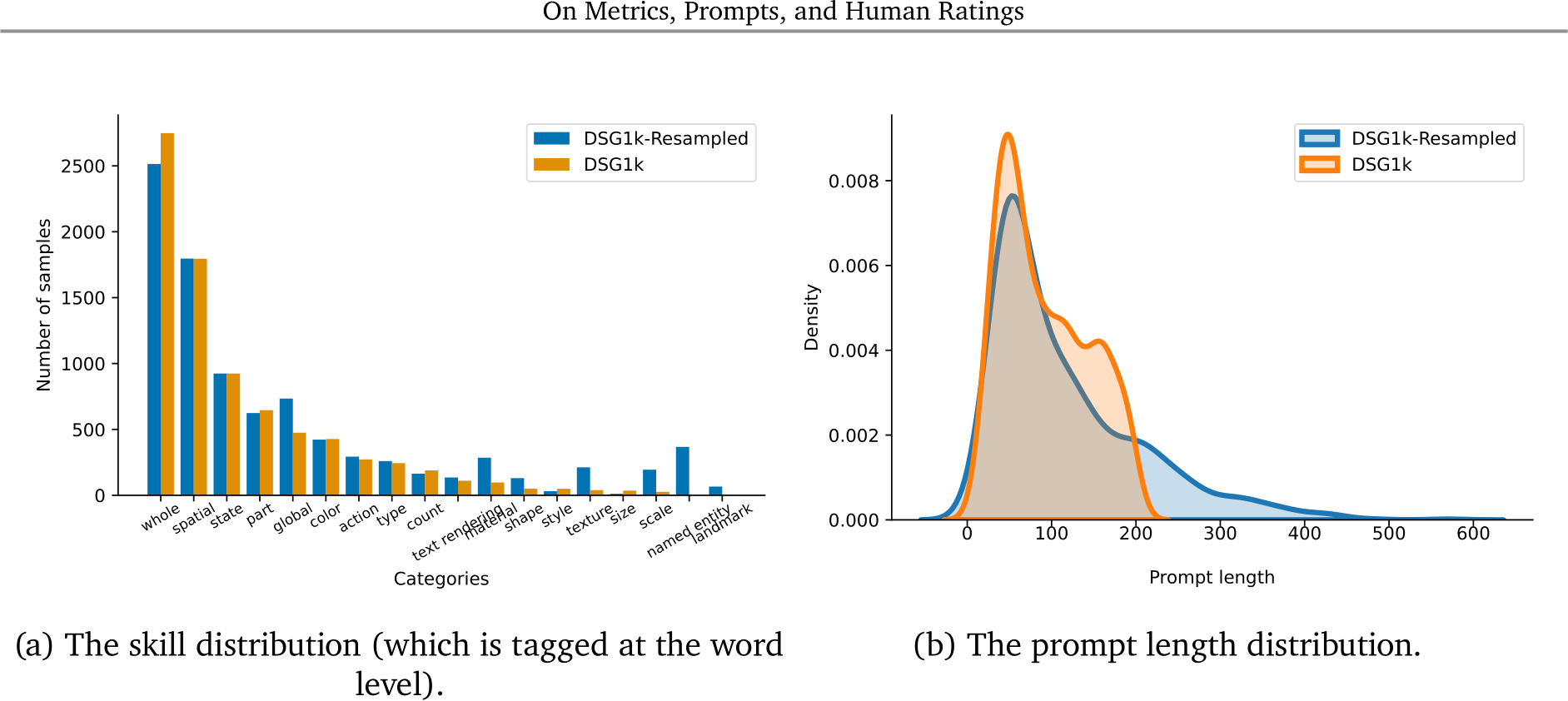
Figure 8 | Prompt distribution in DSG1K-Resampled(Gecko-R) and DSG1K.

length and language (we use English and Gibberish but we note this could be easily extended to more languages). We then create examples that have those properties to create our few-shot prompt. We can query the LLM as many times as we like to create a distribution of prompts across different text lengths and languages. We do a similar setup for each of the skills and sub-skills we define below.

C.4. Breakdown by skill/sub-skill in Gecko(S)

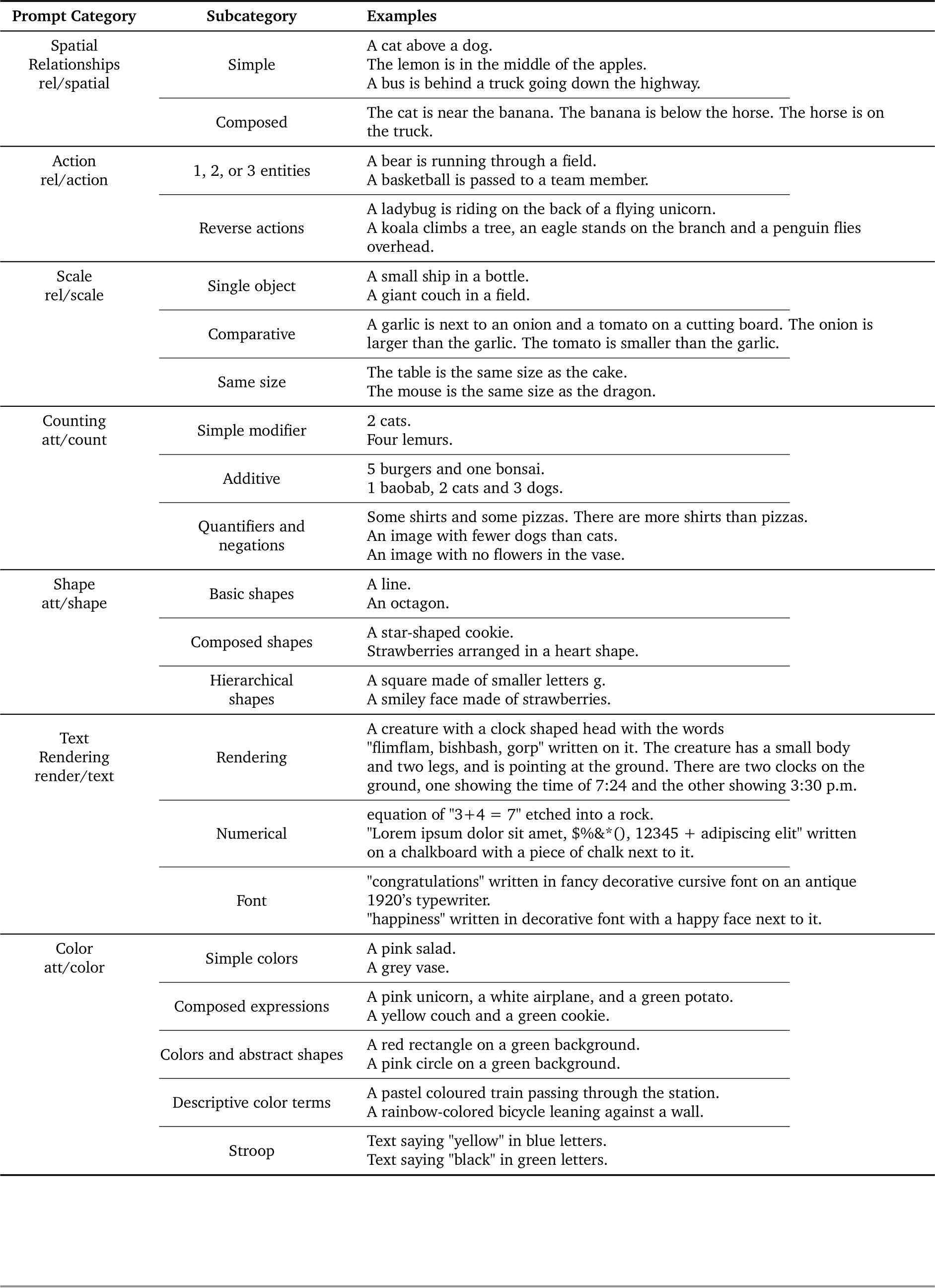
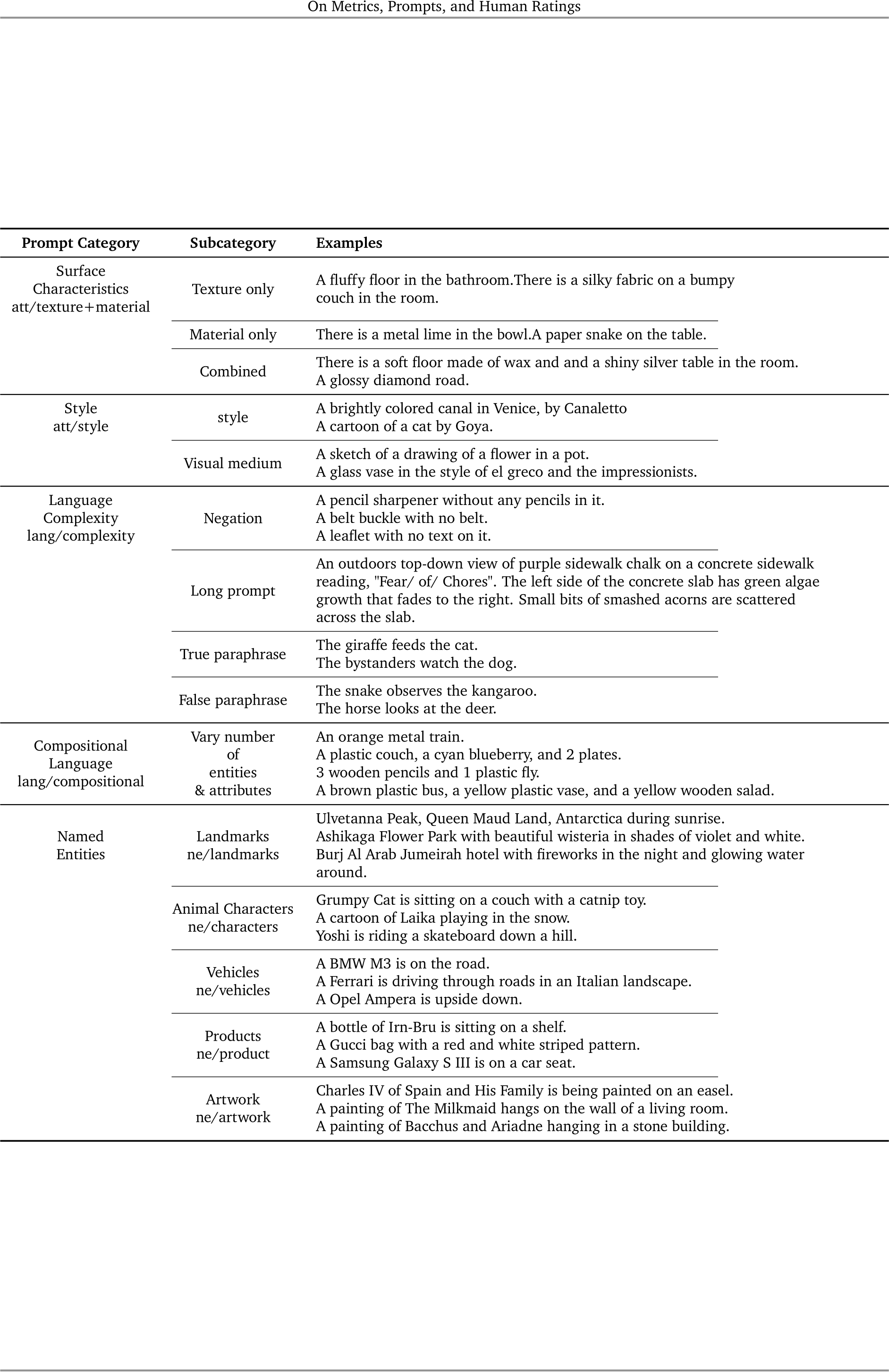
An overview of Gecko(S) is given in Fig. 7. In this section we give more information on the skills and sub-skills within Gecko(S). We provide a detailed breakdown of each prompt sub-skill, including examples and justifications. Skills and sub-skills are listed in Table 7. We aim to cover semantic skills, some of which have already been covered in previous work (e.g.shapes, colors or counts), while further subdividing each skill to capture its different aspects and difficulty levels. By varying the difficulty of the prompts within a challenge we ensure we are testing the models and metrics at different difficulty levels and can find where models and metrics begin to break.

Each skill (such as shape, color, or numerical) is divided into sub-skills, so that prompts within that sub-skill can be distinguished based on difficulty or, if applicable, some other criteria that is unique to that sub-skill (i.e.prompts inspired by literature in psychology). We create a larger number of examples and subsample to create our final 1K set of prompts to be labelled.

C.4.1. Spatial Relationships

This skill captures a variety of spatial relationships (such as above, on, under, far from, etc.) between two to three objects. In the most simple case, we measure a model’s ability to understand common

Table 7 | Breakdown by skill and sub-skill including examples of prompts.

relationships between two objects. The difficulty is increased by combining simpler entities and requiring the ability to reason about implicit relationships. We use an LLM as described in Sec. C.3 to create these prompts, subsample and manually verify prompts are reasonable.

C.4.2. Action

This skill examines whether the model can bind the right action to the right object, including unusual cases where we flip the subject and the object (i.e.Reverse actions). An example of a reverse setup is that we swap the entities in ‘A penguin is diving while a dolphin swims’ and create ‘A penguin is swimming while a dolphin is diving’. We vary the difficulty by increasing the number of entities. We use an LLM as described in Sec. C.3 to create these prompts, subsample and manually verify prompts are reasonable.

C.4.3. Scale

We measure whether the model can reason about scale cues referring to commonly used descriptors such as small, big or massive. To reduce ambiguity, we typically refer to two objects, so that they can be compared in size. We test the ability to implicitly reason about scales by having Comparative prompts that contain several statements about objects, their relations and sizes. We use an LLM as described in Sec. C.3 to create these prompts, subsample and manually verify prompts are reasonable.

C.4.4. Counting

The simplest sub-skill Simple modifier contains a number (digits such as “2”, “3” or numerals such as “two”, “three”) and an entity. When selecting a vocabulary of words, we aimed to include words that occur less frequently in ordinary language (for example, “lemur” and “seahorse” occur less frequently than “dog” and “cat”) [53]. We focus on numbers 1—10, or 1—5 in more complex cases. Complexity is introduced by combining simple prompts containing just one attribute into compositional prompts containing several attributes. For example, simple prompts “1 cat” and “2 dogs” are combined into a single prompt “1 cat and 2 dogs” in the sub-skill Additive. We also test approximate understanding of quantities based on linguistic concepts of many and few in the Quantifiers and negations sub-skill.

C.4.5. Shape

We test for basic and composed shapes, where composed shapes include objects arranged in a certain shape. Hierarchial shapes are of the following type: “The letter H made up of smaller letters S”. This kind of challenge is used to study spatial cognition and the trade-off between global and local attention in literature on higher-order cognition [13]. We use an LLM as described in Sec. C.3 to create these prompts, subsample and manually verify prompts are reasonable.

C.4.6. Text Rendering

We investigate a model’s ability to generate text (both semantically meaningful and meaningless), including text of different lengths. We further test for the ability to generate symbols and numbers, as well as different types of fonts. We use an LLM as described in Sec. C.3 to create these prompts, subsample and manually verify prompts are reasonable.

C.4.7. Colour

The simplest prompts in this skill include basic colours bound to objects. As before, we introduce complexity by combining several simpler prompts (either two or three objects bound with a colour attribute). To include diversity of possible colour attributes, we also test descriptive colour terms such as “pastel” or “rainbow-coloured”. Finally, the sub-skill stroop contains prompts of the type “Text saying "blue" in green letters” similar to the incongruent condition in the Stroop task [55] used to study interference between different cognitive processes.

C.4.8. Surface Characteristics

Surface characteristics include texture and material. We first test for each sub-skill individually, and then combined. Generally, some prompts in this skill can be difficult to visualise as they might include descriptions that are typically of tactile nature (“abrasive” or “soft”).

C.4.9. Style

We divide prompts into two sub-skills: one depicting a style of an artist, and another to capture different visual mediums (such as photo, stained glass or ceramics). We use an LLM as described in Sec. C.3 to create these prompts, subsample and manually verify prompts are reasonable.

C.4.10. Named Entity

This skill evaluates a model’s knowledge of the world through named entities, focusing on specific entity types such as landmarks, artwork, animal characters, products, and vehicles, which are free of personally identifiable information (PII).

For the landmark class, we choose landmarks from the Google Landmarks V2 dataset and ensure we cover different continents and choose landmarks with high popularity [60]. Given this set of landmarks, we use an LLM as described in Sec. C.3 to create these prompts, subsample and manually verify prompts are reasonable.

For the other classes, to curate diverse named entities, we first gather candidates from Wikidata using SPARQL queries. A simple query (e.g., instance of (P31) is painting (Q3305213)) might yield an excessively large number of candidates. Therefore, we impose conditions to narrow down the query responses. See our criteria below.

Artwork : Created before the 20th century; any media; any movement

Animal Characters : Anthropomorphic/fictional animals; real animals with names

Products : Electric devices; food/beverage; beauty/health

Vehicle : Automobiles; aircraft

Once we have a candidate set for each entity class, we focus on selecting reasonably popular entities that are widely recognised and appropriate to present to models. We assess popularity using the number of incoming links to and contributors on their English Wikipedia pages as proxies [18]. Finally, we manually curate the final set of named entities, selecting them based on their ranked popularity scores.

C.4.11. Language complexity

We evaluate models on prompts with “tricky” language structure / wording. For this skill, we include 4 sub-skills: negation, long prompt, and true / false phrases. We sampled 19 prompts for negation from LVIS [21], COCO stuff [6], and MIT Places [68]; 58 true paraphrases and 58 false paraphrases from BLA [9]; and finally crowdsourced 38 for long prompt with the help from English major raters. It should be noted that while we do not cover the entire spectrum of complex language (e.g. passives, coordination, complex relative clausals, etc.), the subcategories included cover the most prominent pain points of image generation models per our experimentation.

We also include a language complexity metric which can be run over all prompts. Here we treat language complexity from two perspectives – semantic and syntactic.

• Semantic complexity. The quantity of semantic elements included in a prompt. • Syntactic complexity. The level of complexity of the syntactic structure of a prompt.

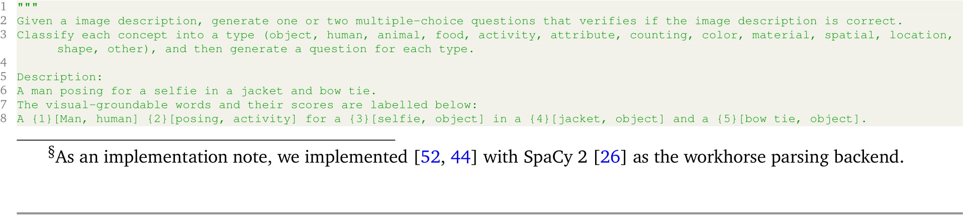
Concretely, we define semantic complexity as the number of entities extracted from a prompt. Taking the visual relevance of the task into account, we apply Stanford Scene Graph Parser [52] for entity extraction and count the number of unique entities as the proxy for semantic complexity. For syntactic complexity, we implement a modified variant of [44] to look for the deepest central branch in the dependency tree of a prompt (pseudo-code below) § to gauge the complexity of its syntactic structure.

D.1. LLM prompting for generating coverage

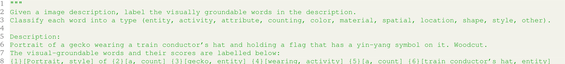
and {7}[holding, entity] {8}[a, count] {9}[flag, entity] that has {10}[a yin-yang symbol, entity] on it. {11}[Woodcut, material].

Listing 3 | LLM sampling template for labelling visually groundable words/phrases.

D.2. LLM prompting for generating QAs

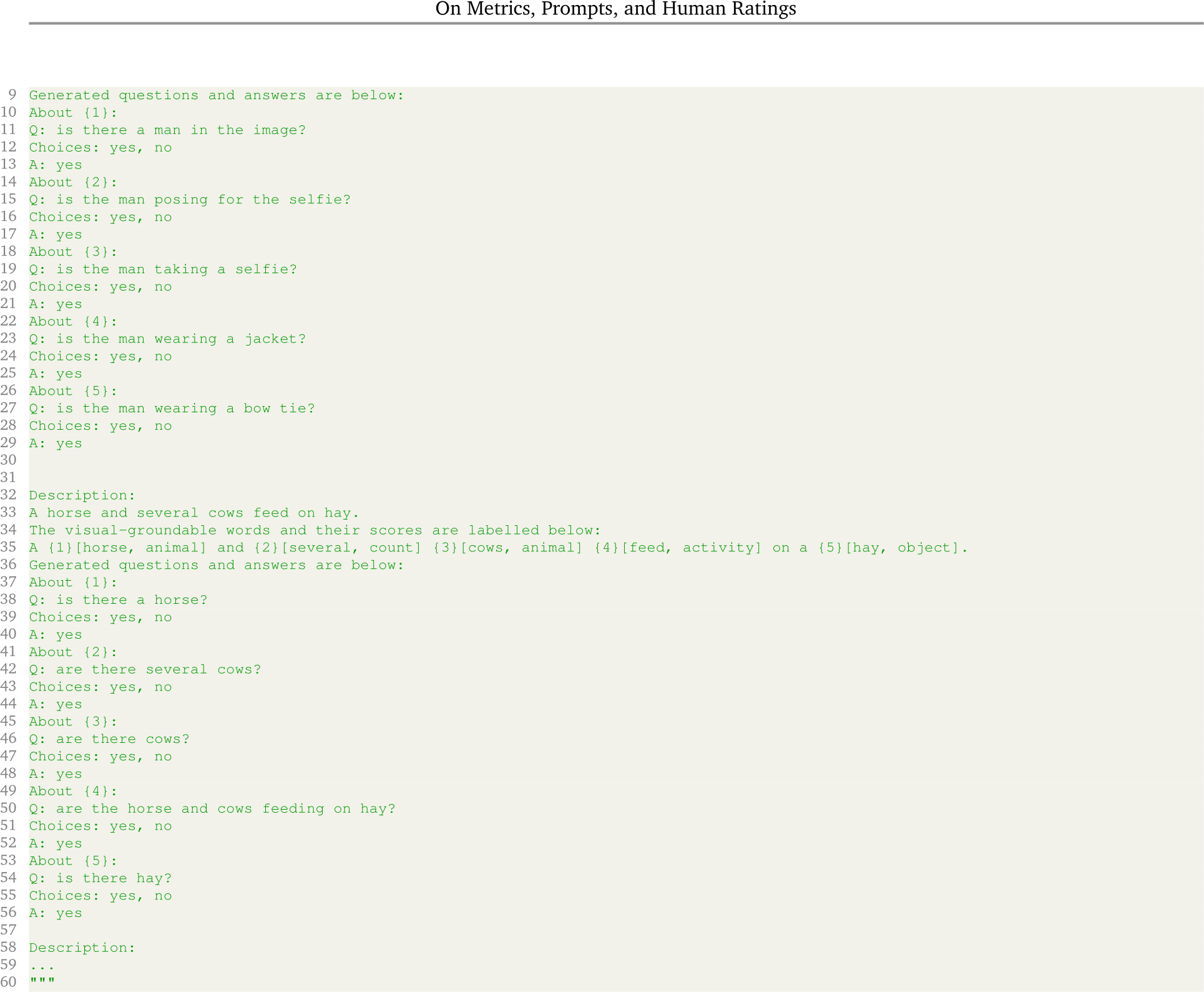
Listing 4 | LLM sampling template for generating QAs.

E.1. Annotation templates

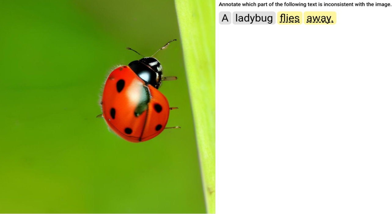
Figure 9 | Word-level annotation template user interface. Example depicting the interface shown to the annotators when performing evaluation tasks with the WL template. Raters are asked to click on words they find are not aligned with image, and double click on the words where they are unsure.

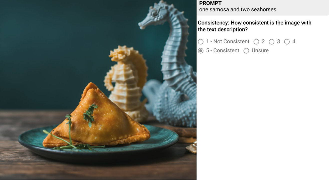
Figure 10 | Likert annotation template user interface. Example depicting the interface shown to the annotators when performing evaluation tasks with the Likert template. Raters are given the prompt and image and asked to rate on a 5-point scale how consistent the image is with respect to the prompt. An Unsure option is also given the annotators.

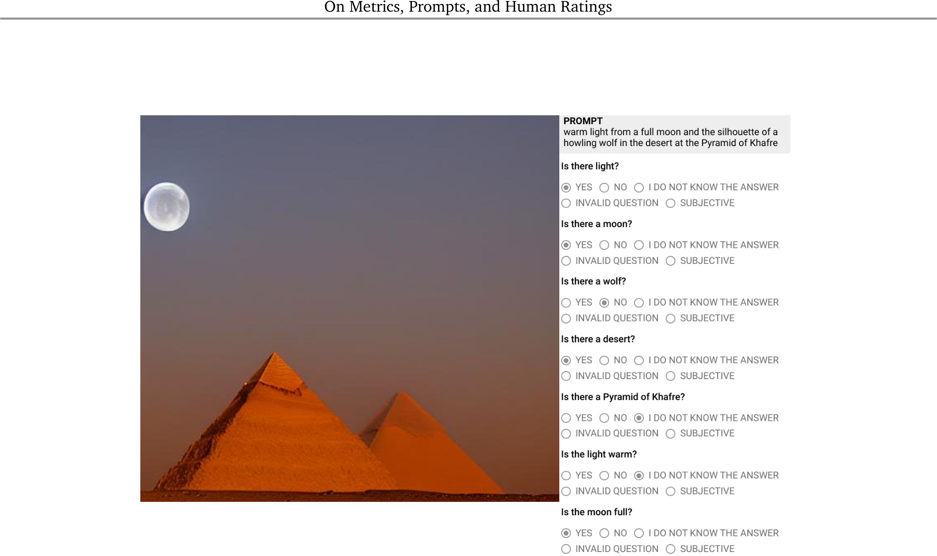
Figure 11 | DSG(H) annotation template user interface. Example depicting the interface shown to annotators when performing evaluation tasks with the DSG(H) template. Raters are given the image, prompt, and respective automatically generated questions. There are 5 options for answering each question. In our analysis, both I do not know the answer and Subjective answers are considered as Unsure.

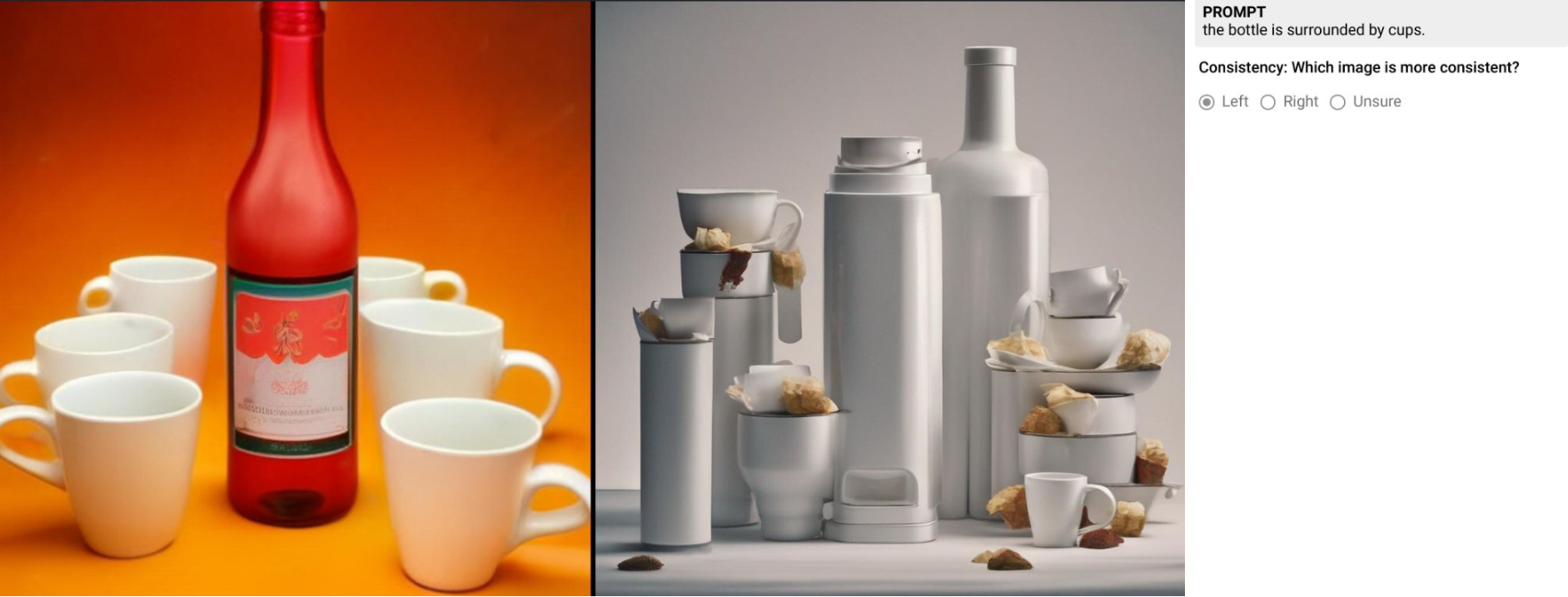
Figure 12 | Side-by-side comparison annotation template user interface. Example depicting the interface shown to the annotators when performing evaluation tasks with the side-by-side template. Raters are given a pair of images from different models, the prompt used to generate them and asked to pick which one is more consistent with the prompt. An Unsure option is also given.

E.1.1. Percentage of unsure ratings for each annotation template/model

One of the innovations of our human evaluation setup is to allow for annotators to reflect uncertainty in their ratings. In Table 8 we show the percentage of Unsure ratings for each absolute comparison annotation template. Overall, we find that evaluations with Gecko(R) yield a higher percentage of Unsure ratings in comparison to Gecko(S).

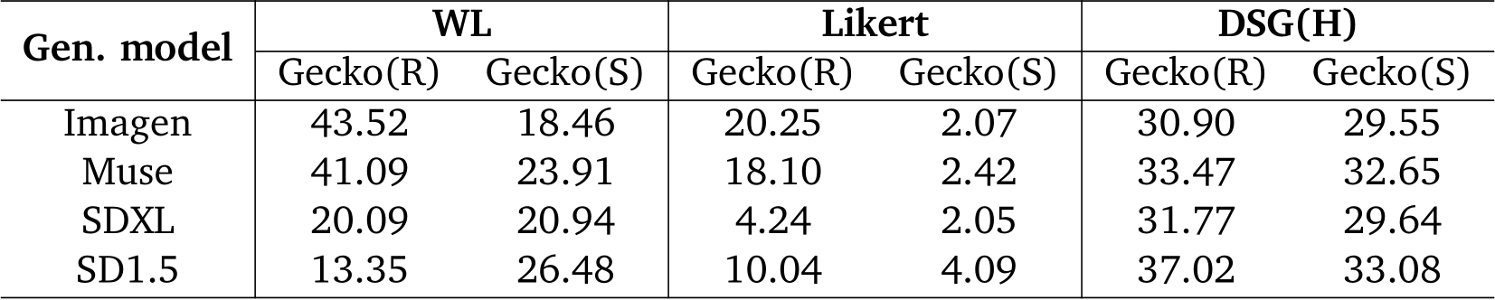
Table 8 | Percentage of Unsure ratings. Overall, evaluation with Gecko(S) yields fewer Unsure ratings across all models and templates.

E.2. Additional experimental results

E.2.1. Correlation across templates and models.

We show the correlation between templates and models for both Gecko(R) and Gecko(S) in Table 9.

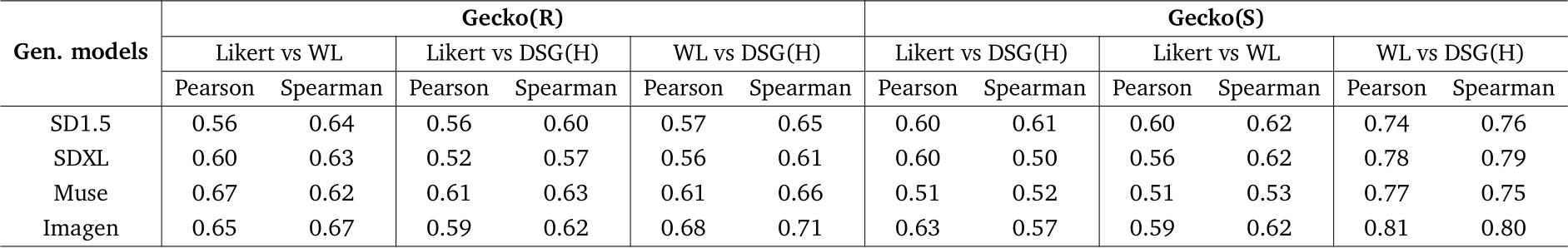
Table 9 | Correlation between all absolute comparison templates. We compute Pearson and Spearman correlation coefficients for all pairs of templates for both Gecko(R) and Gecko(S). We find significant results with 001 for all cases and that scores of all metrics are at least moderately correlated, with the finer-grained templates, WL and DSG(H), being more correlated with each other in comparison to Likert.

E.2.2. Distribution of scores per prompt-image pairs across annotation templates.

We plot the distribution of scores per each evaluated prompt-image pair for all the absolute comparison templates. The violin plots in Fig. 13-14 show the distributions for Gecko(R) and Gecko(S), respectively. It is possible to notice that scores obtained for Muse with WL and DSG(H) are more concentrated in values closer to 1 for both templates, corroborating findings from Sec. 4.3 where results showed Muse was the overall best model.

E.2.3. Side-by-side template.

In Table 10 we show inter-annotator agreement results for the side-by-side annotation template for Gecko(R) and Gecko(S), along with the respective difference in agreement when using only the reliable prompts for both Gecko2K subsets. In Table 11 we present the results of the comparison between the side-by-side template and the absolute comparison ones.

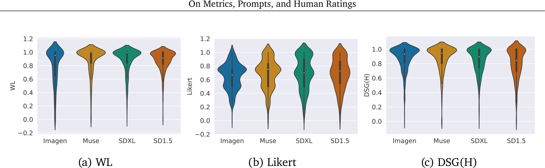
Figure 13 | Distribution of scores for Gecko(R). We show violin plots for scores obtained with all absolute comparison templates.

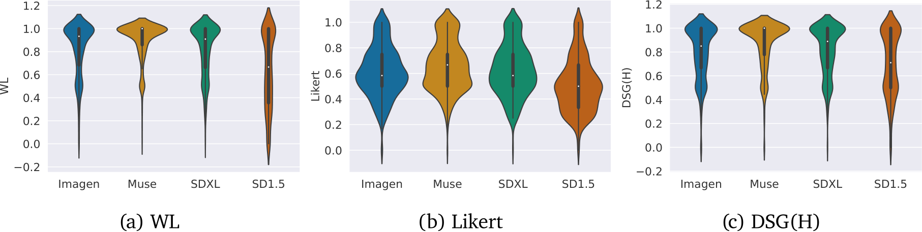
Figure 14 | Distribution of scores for Gecko(S). We show violin plots for scores obtained with all absolute comparison templates.

E.3. Reliable prompts: Examples of image-prompt pairs with high human (dis)agreement

In this section we show a representative list of prompts and corresponding images where human annotators were most likely to either agree or disagree in their ratings. The annotators agreed in ratings if they gave similar scores across for an image-text pair, meaning that the resulting mean variance was zero or close to zero. We refer to such prompts as “high agreement” prompts. In contrast, if annotators gave different ratings for a text-image pair, this would result in higher mean variance and we call such prompts “high disagreement” prompts.

To find prompts with high agreement across raters for all templates and all models, for each model-template combination we pick a subset of responses with low variance. Low variance is defined as the mean variance of a prompt-image pair for a model-template pair being below a certain threshold. The threshold is set as 10% of the maximum variance for that model-template set of ratings for both Gecko(R) and Gecko(S). Analogously, we also find a set of prompts with high disagreement; for this we find prompts that have mean variance above 1% of the maximum variance for a given template and for prompts from Gecko(R) and Gecko(S). The specific threshold value here is relevant only insofar as it captures at least 10 prompt-image pairs which we are interested in visualising. Then, we find prompts with high agreement by intersecting all model-template prompt sets where prompts have been selected based on the threshold. The procedure is analogous for low agreement prompts. For Gecko(R), both sets, namely the set of prompts with high agreement as well as the set of prompts with high disagreement have 34 prompts each. For Gecko(S), the set of prompts with high agreement has 62 prompts, while the set of prompts with high disagreement contains 85 prompts. A subset of 10 prompts for all different combinations is listed in Tables 12-15 and corresponding images are shown in the Figure 15-18.

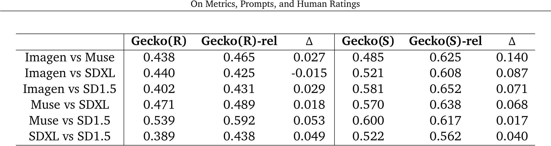
Table 10 | Side-by-side template: inter-annotator agreement. We compute Krippendorff’s for Gecko(R) and Gecko(S) and the difference (when using only reliable prompts for both subsets of Gecko2K. In both cases, using the reliable subsets increases the overall inter-annotator agreement.

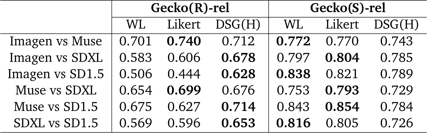
Table 11 | Comparing side-by-side and absolute templates. We compare the side-by-side template with the absolute comparison ones by computing the accuracy obtained by WL, Likert, and DSG(H) scores when using them to compare pairs of images. In this case, the ground-truth is assumed to be the results obtained with the side-by-side template.

Based on the analyses of such subsets, we observe several interesting trends. First, for Gecko(R) the prompts with higher agreement tend to be significantly shorter in length as measured by the number of characters, compared to the length of prompts with high disagreement 17386.35, Welch’s t-test 42 (p<0.001). The same observation holds for Gecko(S), where high agreement prompts were also significantly shorter high disagreement prompts 8295.17, Welch’s t-test 80 (p<0.001). We further observe that prompts where raters tend to agree more are highly specific (i.e.they refer to one or just a few objects with few attributes), whereas prompts with high disagreement tend to describe more complex scenes with visual descriptors and often mentioning named entities or text rendering. Intuitively, this makes sense as longer prompts are more likely to require several skills.

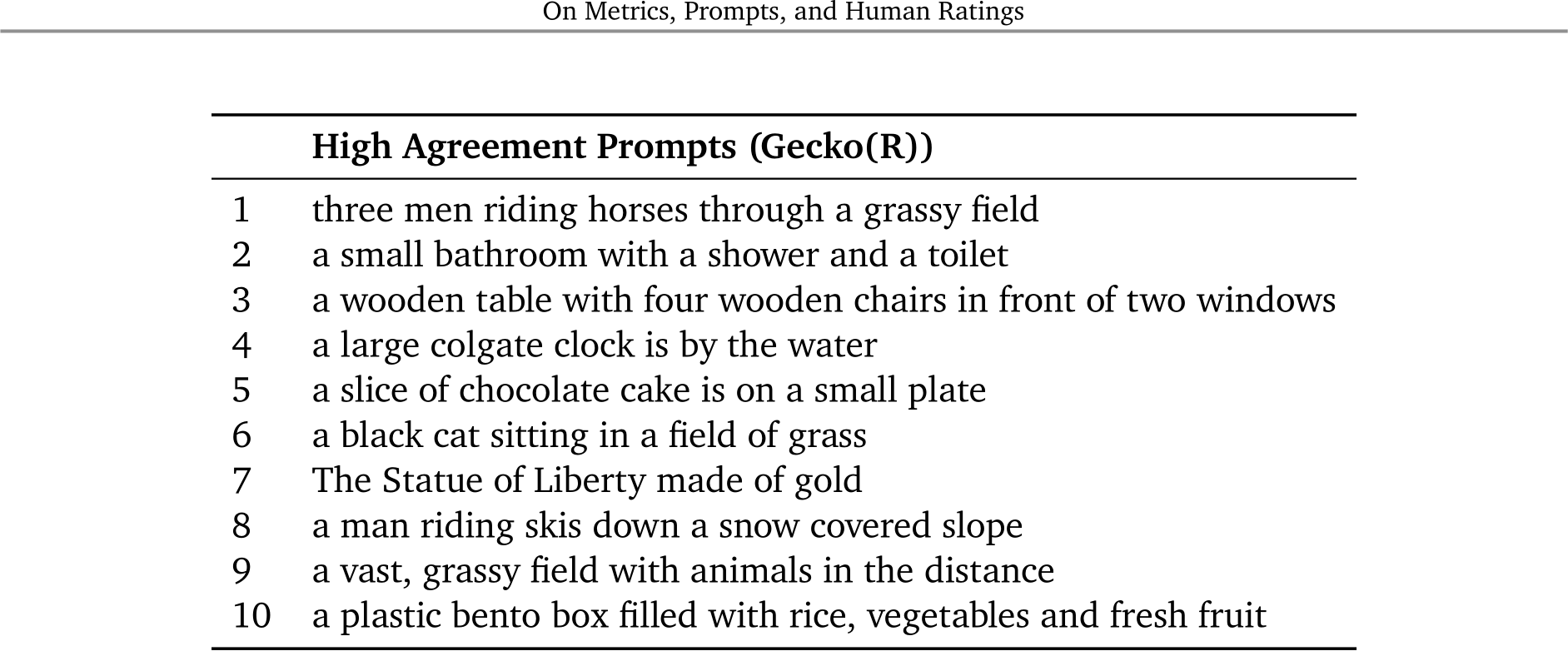
Table 12 | Examples of Gecko(R) reliable prompts. We show examples of Gecko(R) reliable prompts computed with a threshold equal to 10% of maximum disagreement.

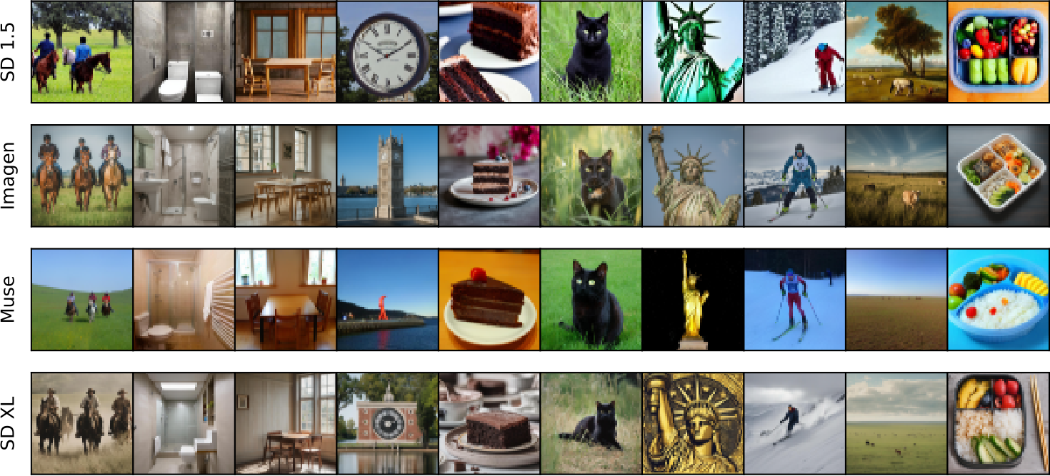
Figure 15 | Images generated with Gecko(R) reliable prompts. We show examples of images obtained with Gecko(S) reliable prompts computed with a threshold equal to 10% of maximum disagreement. Corresponding prompts are shown in Table 12.

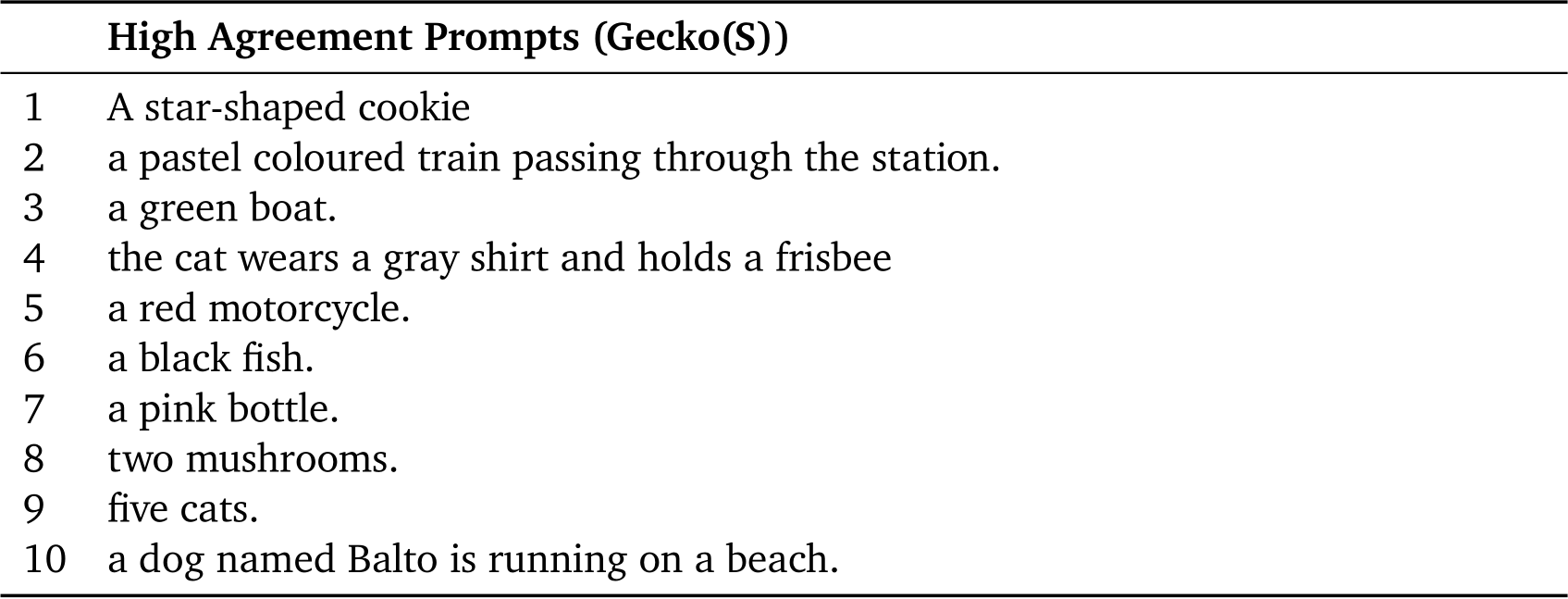
Table 13 | Examples of Gecko(S) reliable prompts. We show examples of Gecko(S) reliable prompts computed with a threshold equal to 10% of maximum disagreement.

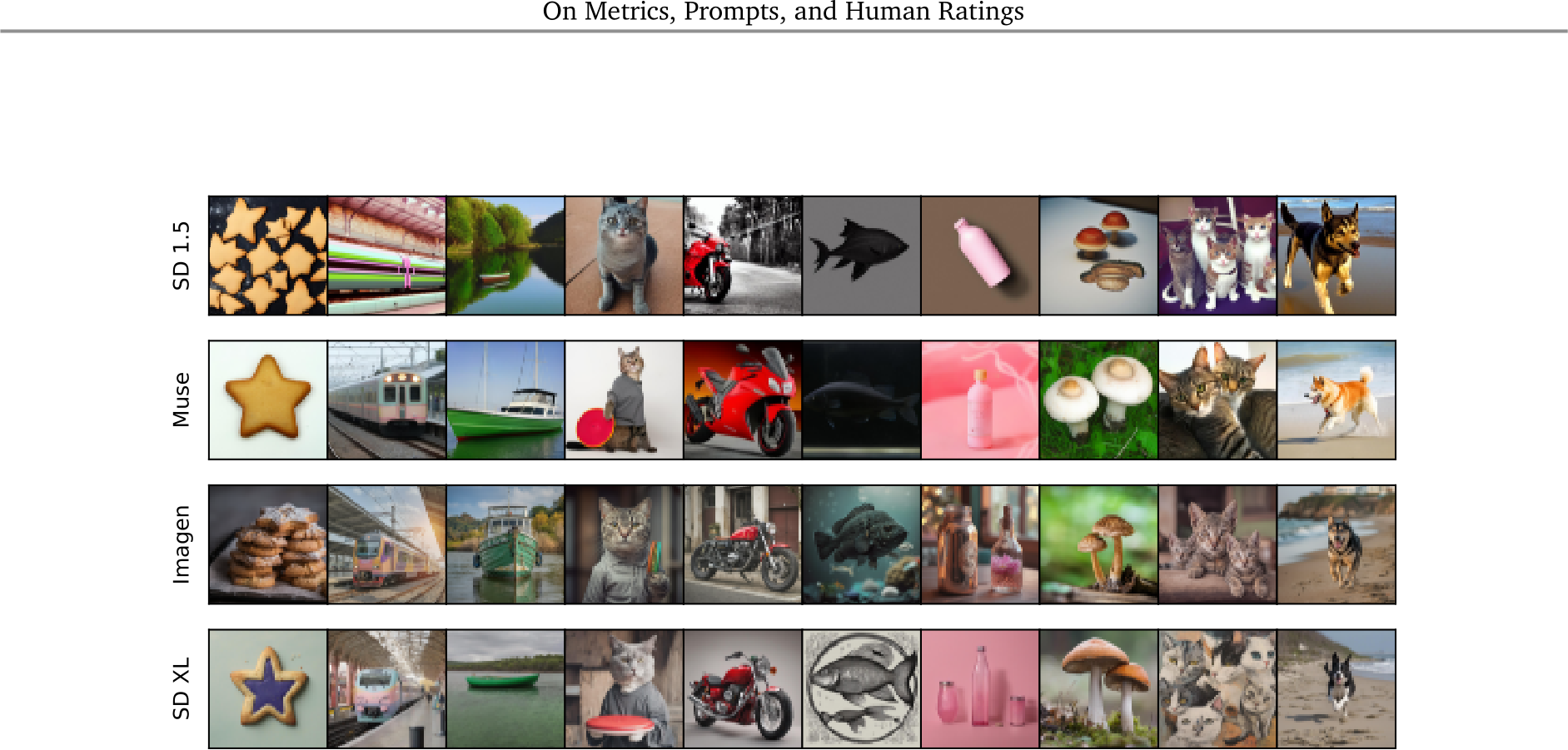
Figure 16 | Images generated with Gecko(S) reliable prompts. We show examples of images obtained with Gecko(S) reliable prompts computed with a threshold equal to 10% of maximum disagreement. Corresponding prompts are shown in Table 13.

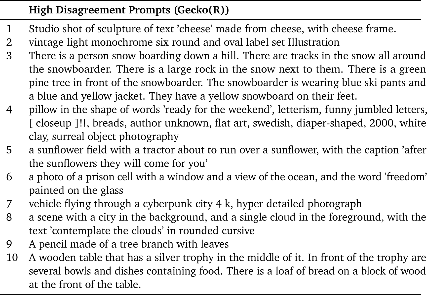
Table 14 | Examples of Gecko(R) non-reliable prompts. We show examples of Gecko(R) non-reliable prompts computed with a threshold equal to 99% of maximum disagreement.

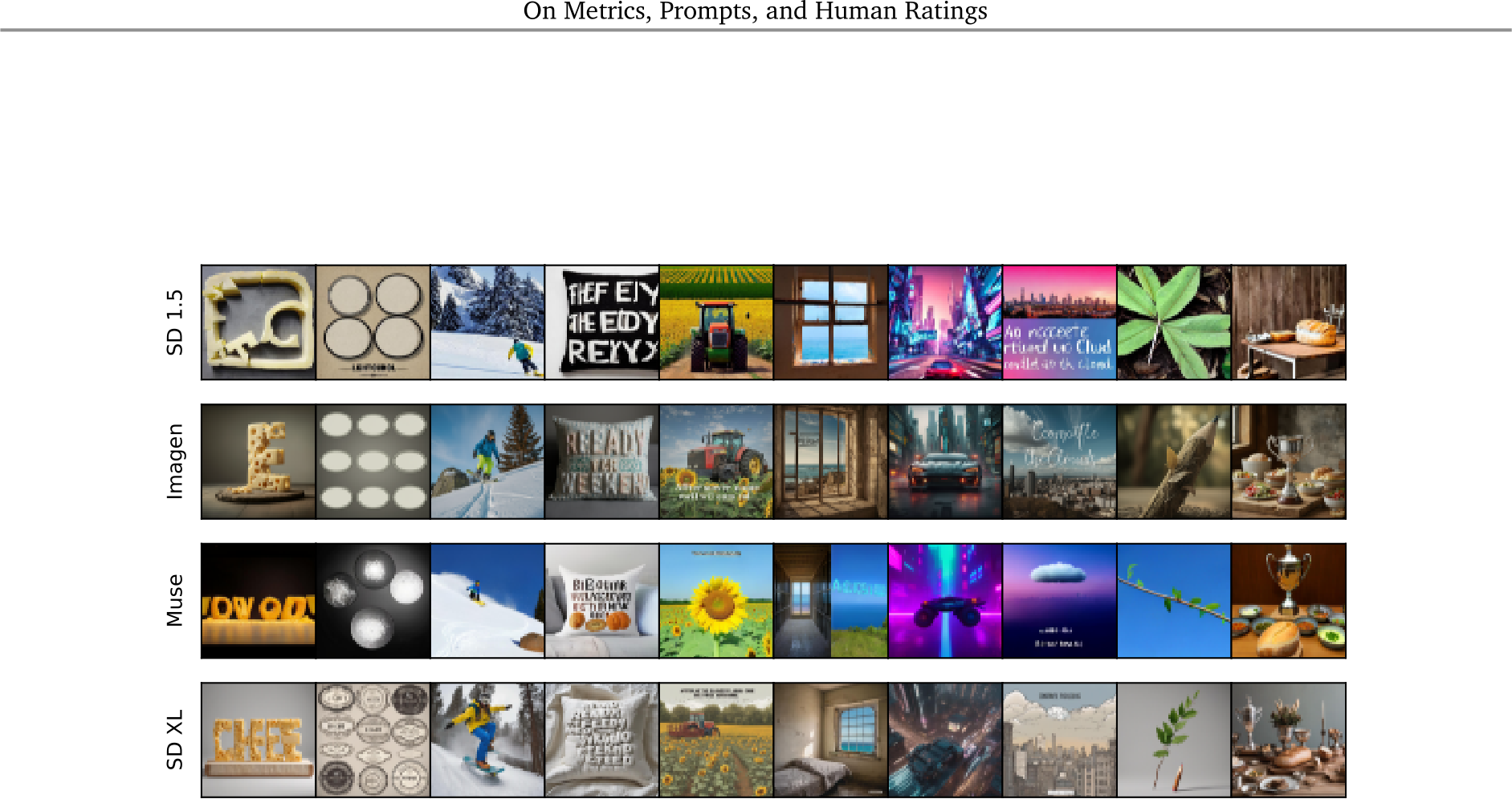
Figure 17 | Images generated with Gecko(R) non-reliable prompts. We show examples of images obtained with Gecko(R) non-reliable prompts computed with a threshold equal to 99% of maximum disagreement. Corresponding prompts are shown in Table 14.

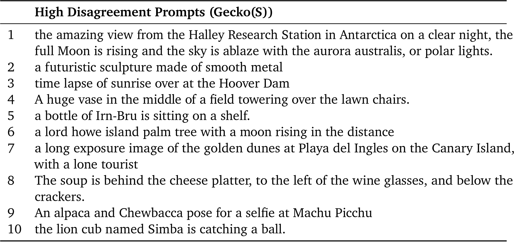
Table 15 | Examples of Gecko(S) non-reliable prompts. We show examples of Gecko(R) non-reliable prompts computed with a threshold equal to 99% of maximum disagreement.

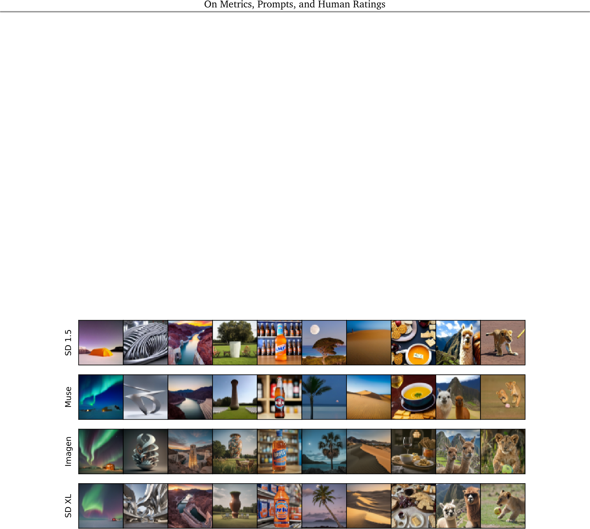
Figure 18 | Images generated with Gecko(S) non-reliable prompts. We show examples of images obtained with Gecko(S) non-reliable prompts computed with a threshold equal to 99% of maximum disagreement. Corresponding prompts are shown in Table 15.

E.4. Human evaluation templates: Challenging cases

In Figs. 19, 20, and 21 we show examples of challenging cases for the absolute comparison templates.

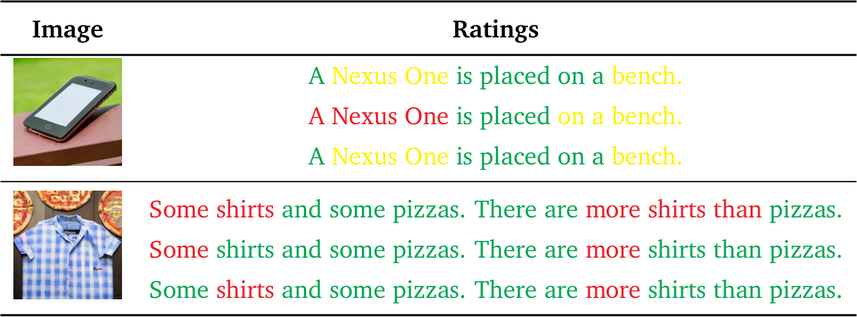
Figure 19 | Examples of challenges for WL. We show two examples of evaluated images, respective prompts and annotations from three raters. Each word is coloured according to the score given by the rater: green indicates Aligned, red Not aligned, and yellow Unsure. Both examples show that WL can be sensitive to words that are not relevant to the alignment evaluation. Top: All raters seem to agree it is not possible to tell whether a bench is represented in the image (hence the word is evaluated as Unsure). In spite of that, one of the raters disagrees on how to rate the “on a” preposition. Bottom: All raters seem to agree the quantity of shirts in the image does not reflect the prompt, but their ratings vary in terms of which words are rated as not aligned.

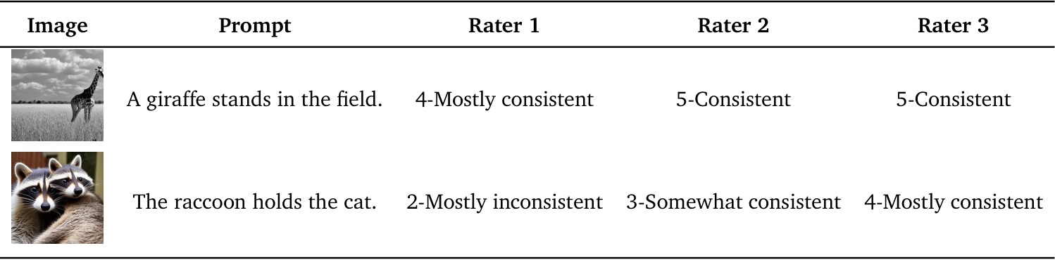
Figure 20 | Examples of challenges for Likert. Top: Raters might take into account other aspects of the images besides alignment when evaluating a prompt-image pair. In this example, although the image is perfectly consistent with the prompt, one of the raters penalised its score. We hypothesise they took into account the fact the generated image is in grey scale. Bottom: “Uncalibrated” scores across raters. The scores of all three raters reflect the imperfect consistency between prompt and image, but each rater penalised the score with different intensity.

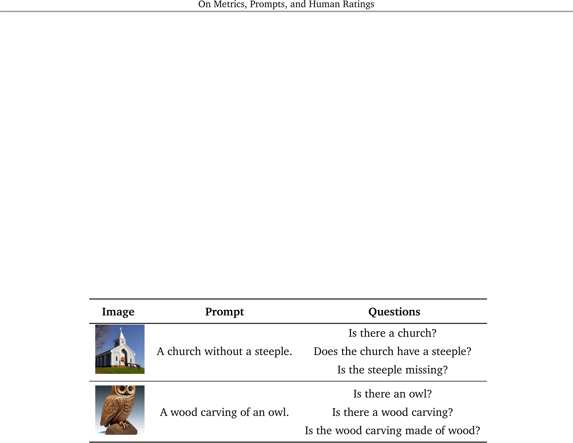
Figure 21 | Examples of challenges for DSG(H). Top: Language complexity–Negation. As also shown in Fig. 6, the question generation is confused by the negation (asking if the church has a steeple as opposed to does not have a steeple). Bottom: Coverage. The question generation fails to capture that the owl should be represented as a wood carving.

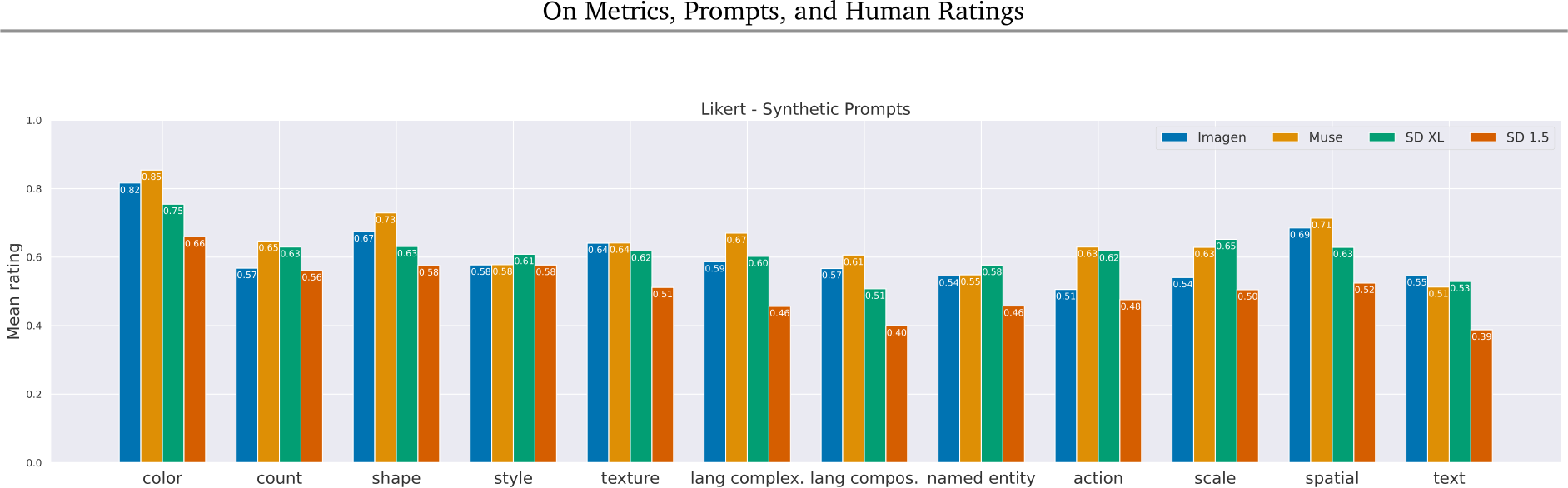
Figure 22 | Per skill results - Likert. Muse scores the best in nine out of the twelve categories, and SD1.5 performs the worst in all categories. Focusing on Muse, SDXL, and Imagen, the models score above 0.5 on all categories. Recalling that the Likert scale is symmetric (0.0 being inconsistent, and 1.0 being consistent), we see that these three models are more consistent than inconsistent on average (albeit only slightly for skills such as ‘lang compos.’ – , ‘named entity’ and ‘text’).

F.1. Analysing Model Ratings Per Skill

In Figures 22, 23 and 24, we plot the mean ratings in different skills for Likert, WL and DSG(H), respectively. We focus on Gecko(S) because we have a skill/sub-skill label for each prompt. Our goal is to understand how the trends in model performance on the whole prompt set relate to their performance in individual skills. We provide an overview of the results in the captions for the plots. Overall, the results broken down by skill are consistent with the averages over the whole prompt set. In other words, if a model is better or worse on the full prompt set, this is generally true for the individual categories as well. Another observation is that counting and complex language seem to be the most difficult skills judging by WL and DSG, but this is not as clear from Likert (where many categories seem just as difficult).

Further Breaking Down Skills. We can gain more insight into the skills of the models by looking at variation within a skill. Figure 25 shows sub-skills of the colour prompts. Two sub-skills are more challenging: the prompts require the models to combine multiple skills when generating the image (colour plus either composition or text rendering). The ‘colour:composed’ sub-skill (composed expressions) includes prompts such as ‘A brown vase, a white plate, and a red fork.’ with variations in the colors/objects. The sub-skill ‘color:stroop’ (stroop) contains prompts like ‘Text saying "green" in white letters.’ where the word in quotes differs from the color of the letters.

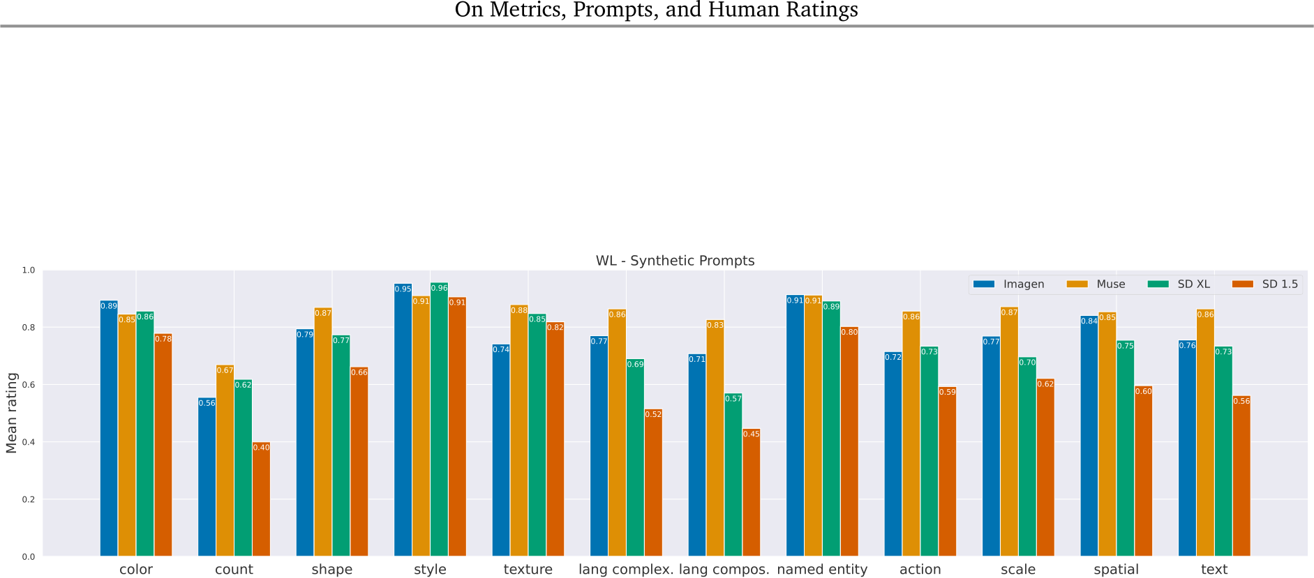
Figure 23 | Per skill results - WL. Muse scores the best in ten out of the twelve skills, and SD1.5 performs the worst in all skills. Moreover, Muse scores higher than the other models by a noticeable margin (for the skills ‘lang compos.’, ‘action’, ‘scale’ and ‘text’. In this case, analysing the results by skill shows that we can contribute Muse’s higher average score (over the whole prompt set) mostly to these skills.

0.86 0.89 0.88 0.880.86

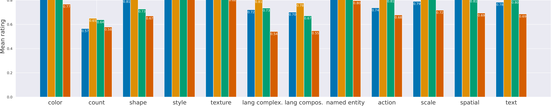
Figure 24 | Per skill results - DSG(H). Muse performs well across the skills, being the best eleven out of twelve times (scoring very close to the top for ‘style’). On the other hand, SD1.5 scores the worst in all the skills. This is consistent with the average scores on the overall prompt set. We see that counting is the most difficult skill for Muse, SDXL, and Imagen. Aside from counting, the hardest skills for Muse are the language ones (‘lang complex.’ and ‘lang compos.’). This relative skill deficiency is not evident from the Likert and WL ratings, and therefore, the DSG ratings are better able to capture model shortcomings for prompts with more complex linguistic structure.

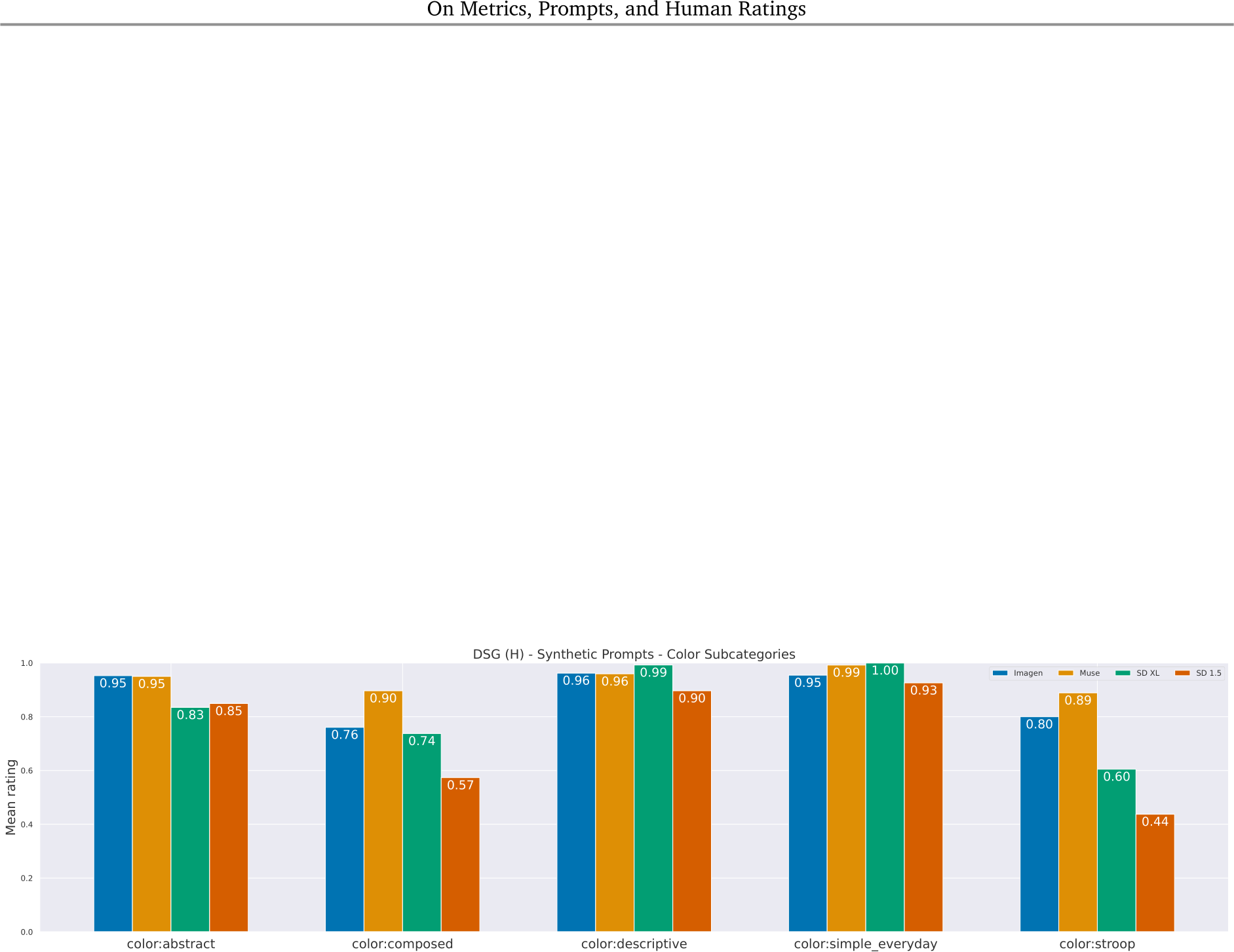
Figure 25 | Color sub-skill results - DSG (H). We further break down the prompts in the color skill into five sub-skills. One observations is that two of the sub-skills (‘composed’ and ‘stroop’) are noticeably more difficult for all the models. This can be explained by the fact that they combine multiple skills: ‘composed’ includes prompts with multiple colors/objects, and ‘stroop’ includes text rendering in a certain color. Hence, while models may perform well on a skill overall, the sub-skills can illuminate where they struggle in generating images aligned with more complex prompts. On the other hand, models perform well with both abstract and everyday colors, likely because these are more commonly seen during training.

F.2. Model comparisons with TIFA160

We augment the experiment from Fig. 4 in Sec. 4.3 by performing a similar analysis with TIFA160. We generate images with this set of prompts and perform human evaluation following the same protocol as for Gecko2K and its subsets. In Fig. 26, we show the results of pairwise model comparisons with TIFA160 carried out with the Wilcoxon signed-rank test with 001. Results show that all three versions of Gecko prompts are able to better distinguish models by finding more significant comparisons between them.

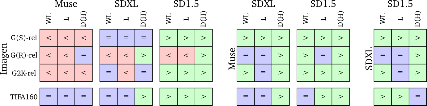
Figure 26 | Comparing models using human annotations. We compare model rankings on the reliable subsets of Gecko(S) (G(S)-rel), Gecko(R) (G(R)-rel), both subsets (G2K-rel), and TIFA160. We perform the Wilcoxon signed-rank test for all pairs of models (p<0.001) and post-hoc comparison based on average ratings. Each grid represents a comparison between two models. Entries in the grid depict results for WL, Likert (L), and DSG(H) (D(H)) scores. The > sign indicates the left-side model is better, worse (<), or not significantly different (=) than the model on the top. All three versions of Gecko prompts are able to better distinguish models by finding more significant comparisons between them.

G.1. Pearson correlation Gecko2K.

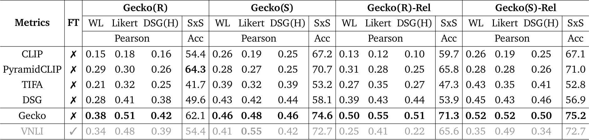
Table 16 | Pearson correlation between VQA-based, contrastive, and fine-tuned (FT) auto-eval metrics and human ratings across annotation templates on Gecko2K and Gecko2K-Rel. Similar to the comparisons on Spearman correlation, Gecko again outperforms other auto-eval metrics with higher overall Pearson correlation.

We report the Spearman Rank correlation of different auto-eval metrics on Gecko2K in 4, here we report the Pearson correlation in 16 as well.

G.2. Model-ordering Evaluation

We provide detailed results for the model ordering experiment in Sec. 6.3. The goal is to examine if each auto-eval metric can predict how two models are ordered according to the human ratings. We use the results obtained by comparing T2I models with scores from all absolute comparison templates reported in Fig. 4 and consider the majority relation assigned to a model pair as the ground truth: if two of the templates find model 1 is better than model 2, then we assume model 1 > model 2. We notice that in all comparisons at least two templates agree in their results, always making it possible to define a ground-truth. We then count the number of times an auto-eval metric successfully found the same relation, in terms of both significance and direction. In addition, we count the number of times an auto-eval metric captured the ground-truth relationship following the most common practice in the literature: ordering models by solely comparing the mean values of scores regardless of statistical significance.

In Figs. 27 and 28, we show the results for all auto-eval metrics on both Gecko(R) and Gecko(S), respectively. Results highlight that the number of significant successful comparisons is lower than comparisons with mean values. All metrics except for DSG and CLIP get the same number of successful comparisons for both criteria. Note that Gecko not only is within the metrics that best capture pairwise model orderings as per the human evaluation ground-truth values, but Gecko scores are also the best correlated with the human scores themselves (as we can see in Table 4).

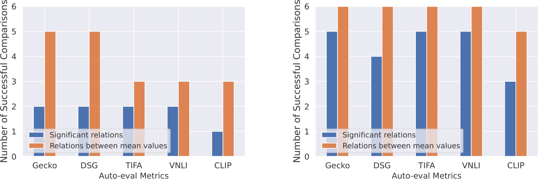
Figure 27 | Gecko(R)-rel: Comparing correct relations between models captured by auto-eval metrics. The ground-truth to computed the number of successful relations is given by human annotation scores.

Figure 28 | Gecko(S)-rel: Comparing correct relations between models captured by auto-eval metrics. The ground-truth to computed the number of successful relations is given by human annotation scores.

G.3. Results for Additional Metrics on the Gecko Benchmark

We compare the Gecko metric with several score-based auto-eval metrics [36, 31, 62, 56, 67, 16, 66], as well as QA-based metrics such as TIFA [29] and DSG [10], and NLI models [61] in Tab. 17.

Generally, our Gecko metric outperforms the others and shows a higher correlation with most of the human annotation templates. DSG is the second best metric, except on SxS where it ranks third. It outperforms TIFA by a clear margin but falls behind Gecko. Finally, we note that Gecko even shows higher correlation than the supervised VNLI model.

Looking at efficient, score-based metrics, we find that PyramidCLIP achieves competitive correlations. Moreover, a larger pre-training corpus leads to better metrics; e.g., as seen by comparing CLIP-B/32 (trained on 400M images) and CLIP-B/32LAION-2B (trained on 2B images). Finally, larger

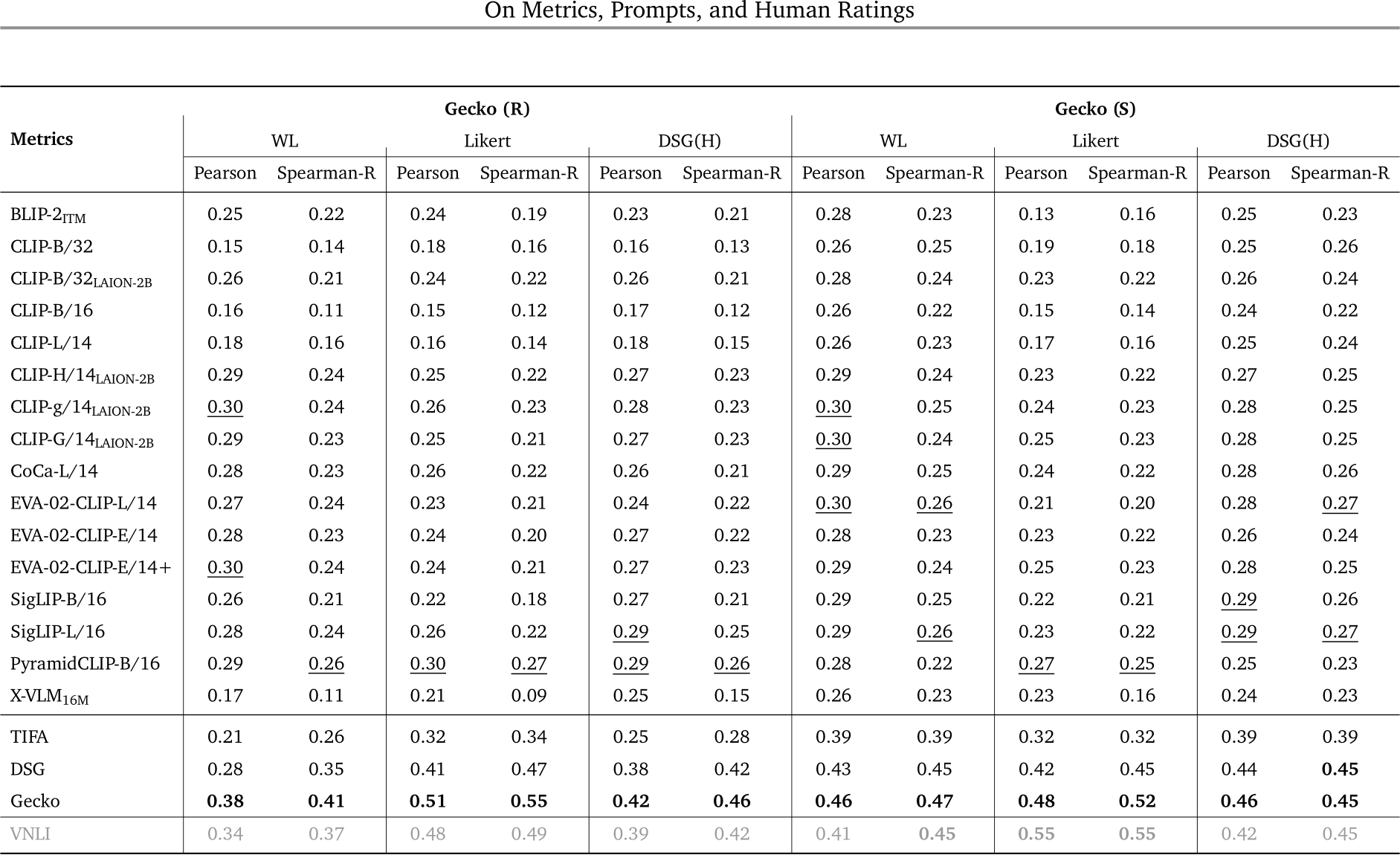
Table 17 | Correlation between auto-eval metrics and human ratings across three annotation templates on Gecko2K. Best results per model type are underlined; best results are in bold.

models are often better (e.g., SigLIP-L/16 vs. SigLIP-B/16), although these trends are less consistent (e.g., EVA-02-CLIP-L/14+ EVA-02-CLIP-E/14).

G.4. Analysing Auto-Eval Metric results per skill.

We present the per-skill Spearman Ranked Correlation between different auto-eval metrics and human annotation templates in 29. We observe a similar trend across the three plots, as we discussed in 6: Gecko is the best on handling prompts with “language complexity”, which can be attributed to the coverage tagging and filtering steps in its pipeline that make Gecko less prone to errors when processing long and complicated prompts. DSG is better on “compositional prompts”, as it can leverage its utilization of dependency graphs. VNLI demonstrates advantages in assessing “shape”, “color”, and “text” (e.g.text rendering) prompts, as the model is trained to discriminate keywords within these categories. Meanwhile, it is also worth noting that all metrics exhibit relatively poor performance on “text” and “named identity”, highlighting the current lack of OCR and named recognition ability in existing contrastive, NLI and VQA models.

G.5. Additional visualisations.

We visualise additional examples in Fig. 30 for different categories (spatial, counting, text rendering, linguistic complexity, etc.). These examples demonstrate both differences arising from different annotation templates and also different metrics.

G.6. Results per Word for WL

Here we evaluate how well the Gecko metric can identify whether words are or are not grounded as rated by WL. This experiment can only be done for Gecko as no other metric gives word level

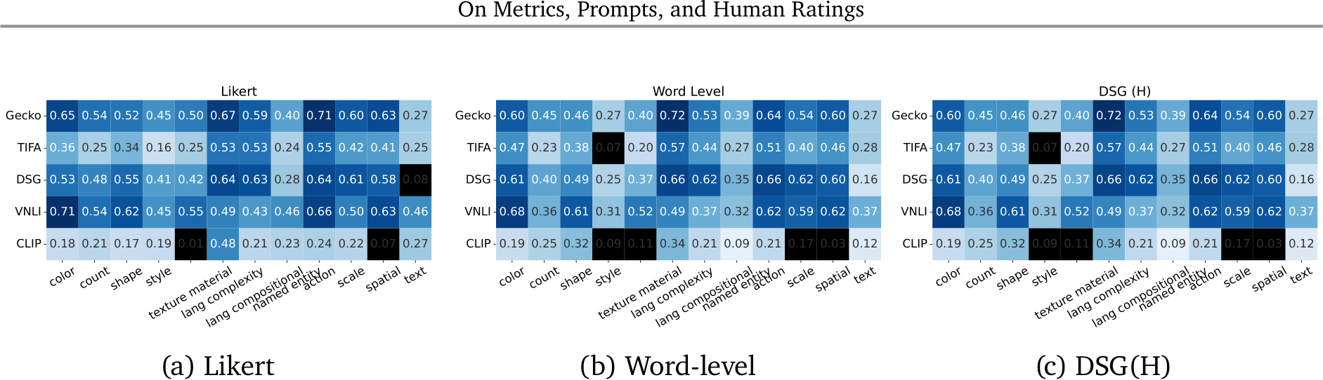
Figure 29 | Per skill results by metric. We visualise the correlation for each skill. Where p-values are > 0.05, we color the square black.

annotations that can be traced back to the original words in the prompt. We note that this is much more challenging than giving an overall image rating. In order to perform this experiment, we first parse the coverage prediction to ensure we can match words in the original prompt with those in the coverage prediction. For example, if we have the original prompt ‘a red-colored dog’ and ‘a {1}[red-colored] {2}[dog]’ as the generated coverage one, we can map from the word index (e.g.‘{1}’ to the phase ‘red-colored’).

We then take all word level predictions where all annotators either annotated the word as grounded or not grounded (we removed those for which a subset of annotators annotated the word as ‘unsure’). For these words, we take the ones where the coverage model predicts that it should be covered (e.g.in the example above, even if ‘a’ was always annotated as grounded, we would ignore it as it is not considered groundable by the coverage step). Given this final set of words, we look at whether the VQA prediction was accurate and compare this to whether the annotators thought that the word was grounded or not.

We report three numbers in Table 18: (1) the number of words we are left with, (2) the accuracy and (3) the error consistency [17], equation (1),(3). We report error consistency as many of the words (90%) are rated as grounded. Accuracy does not account for the fact that a metric which predicts ‘grounded’ 90% of the time would actually get 80% accuracy by chance. Error consistency takes this into account such that 1 means that two sets of results never agree, 0 that the overlap is explained by chance and 1 means results agree perfectly. As shown by the results, Gecko is able to predict grounding at the word level with reasonable accuracy. Moreover, results are not simply explained by chance (as ); the error consistency results indicate in general some but not substantial agreement.

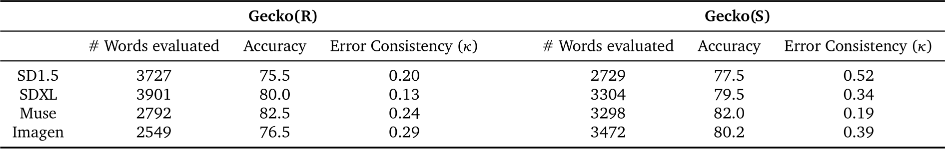
Table 18 | Word level results comparing Gecko to the WL annotation template. We can see that Gecko achieves high accuracy but also that results are not simply explained by chance, as in general indicates fair agreement.

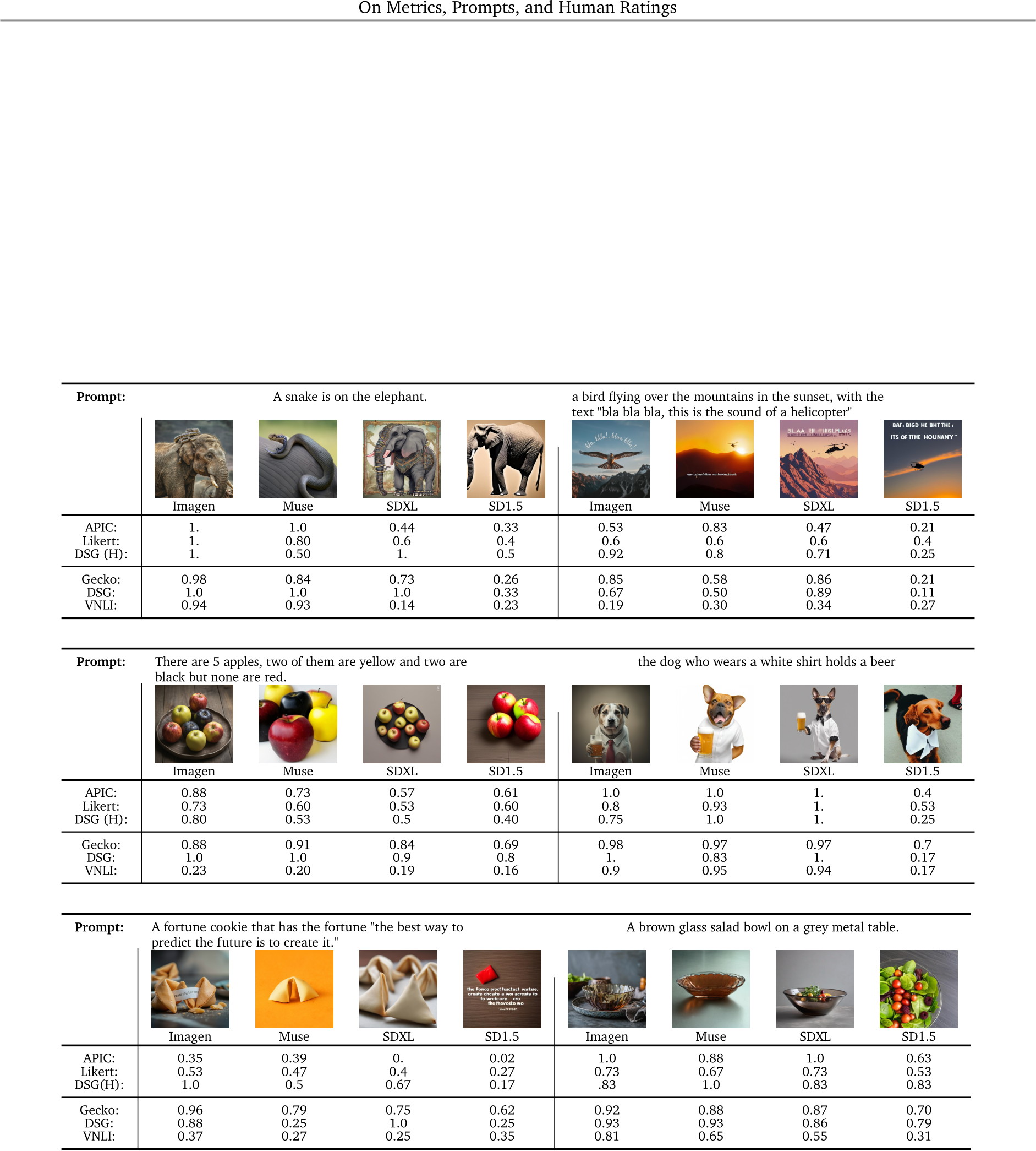
Figure 30 | Additional visualisations of scores from different auto-eval metrics. We show the image generations by the four generative models given two prompts from Gecko(S), with the alignment scores predicted by human annotators and auto-eval metrics respectively.

[1] Anil, R., Dai, A.M., Firat, O., Johnson, M., Lepikhin, D., Passos, A., Shakeri, S., Taropa, E., Bailey, P., Chen, Z., et al.: Palm 2 technical report. arXiv preprint arXiv:2305.10403 (2023)

[2] Bang, Y., Cahyawijaya, S., Lee, N., Dai, W., Su, D., Wilie, B., Lovenia, H., Ji, Z., Yu, T., Chung, W., et al.: A multitask, multilingual, multimodal evaluation of chatgpt on reasoning, hallucination, and interactivity. arXiv preprint arXiv:2302.04023 (2023)

[3] Betker, J., Goh, G., Jing, L., Brooks, T., Wang, J., Li, L., Ouyang, L., Zhuang, J., Lee, J., Guo, Y., et al.: Improving image generation with better captions. Computer Science. https://cdn. openai. com/papers/dall-e-3. pdf 2(3), 8 (2023)

[4] Bitton-Guetta, N., Bitton, Y., Hessel, J., Schmidt, L., Elovici, Y., Stanovsky, G., Schwartz, R.: Breaking common sense: Whoops! a vision-and-language benchmark of synthetic and compositional images. In: ICCV (2023)

[5] Bugliarello, E., Sartran, L., Agrawal, A., Hendricks, L.A., Nematzadeh, A.: Measuring progress in fine-grained vision-and-language understanding. arXiv preprint arXiv:2305.07558 (2023)

[6] Caesar, H., Uijlings, J., Ferrari, V.: Coco-stuff: Thing and stuff classes in context. In: Computer vision and pattern recognition (CVPR), 2018 IEEE conference on. IEEE (2018)

[7] Chang, H., Zhang, H., Barber, J., Maschinot, A., Lezama, J., Jiang, L., Yang, M.H., Murphy, K.P., Freeman, W.T., Rubinstein, M., Li, Y., Krishnan, D.: Muse: Text-to-image generation via masked generative transformers. In: Krause, A., Brunskill, E., Cho, K., Engelhardt, B., Sabato, S., Scarlett, J. (eds.) Proceedings of the 40th International Conference on Machine Learning. Proceedings of Machine Learning Research, vol. 202, pp. 4055–4075. PMLR (23–29 Jul 2023), https://proceedings.mlr.press/v202/chang23b.html

[8] Chen, X., Wang, X., Changpinyo, S., Piergiovanni, A., Padlewski, P., Salz, D., Goodman, S., Grycner, A., Mustafa, B., Beyer, L., Kolesnikov, A., Puigcerver, J., Ding, N., Rong, K., Akbari, H., Mishra, G., Xue, L., Thapliyal, A., Bradbury, J., Kuo, W., Seyedhosseini, M., Jia, C., Ayan, B.K., Riquelme, C., Steiner, A., Angelova, A., Zhai, X., Houlsby, N., Soricut, R.: Pali: A jointly-scaled multilingual language-image model. arXiv preprint arXiv:2209.06794 (2022)

[9] Chen, X., Fernández, R., Pezzelle, S.: The bla benchmark: Investigating basic language abilities of pre-trained multimodal models. In: Proceedings of the 2023 Conference on Empirical Methods in Natural Language Processing. pp. 5817–5830 (2023)

[10] Cho, J., Hu, Y., Garg, R., Anderson, P., Krishna, R., Baldridge, J., Bansal, M., Pont-Tuset, J., Wang, S.: Davidsonian scene graph: Improving reliability in fine-grained evaluation for text-image generation. arXiv preprint arXiv:2310.18235 (2023)

[11] Cho, J., Zala, A., Bansal, M.: Dall-eval: Probing the reasoning skills and social biases of text-to-image generation models. In: ICCV (2023)

[12] Clark, E., August, T., Serrano, S., Haduong, N., Gururangan, S., Smith, N.A.: All that’s ‘human’ is not gold: Evaluating human evaluation of generated text. In: Zong, C., Xia, F., Li, W., Navigli, R. (eds.) Proceedings of the 59th Annual Meeting of the Association for Computational Linguistics and the 11th International Joint Conference on Natural Language Processing (Volume 1: Long Papers) (2021)

[13] Delis, D.C., Robertson, L.C., Efron, R.: Hemispheric specialization of memory for visual hierarchical stimuli. Neuropsychologia 24(2), 205–214 (1986)

[14] Delmas, G., Weinzaepfel, P., Lucas, T., Moreno-Noguer, F., Rogez, G.: Posescript: 3d human poses from natural language. In: ECCV (2022)

[15] Dosovitskiy, A., Beyer, L., Kolesnikov, A., Weissenborn, D., Zhai, X., Unterthiner, T., Dehghani, M., Minderer, M., Heigold, G., Gelly, S., et al.: An image is worth 16x16 words: Transformers for image recognition at scale. arXiv preprint arXiv:2010.11929 (2020)

[16] Gao, Y., Liu, J., Xu, Z., Zhang, J., Li, K., Ji, R., Shen, C.: Pyramidclip: Hierarchical feature alignment for vision-language model pretraining. In: NeurIPS (2022)

[17] Geirhos, R., Meding, K., Wichmann, F.A.: Beyond accuracy: quantifying trial-by-trial behaviour of cnns and humans by measuring error consistency. Advances in Neural Information Processing Systems 33, 13890–13902 (2020)

[18] Geva, M., Khashabi, D., Segal, E., Khot, T., Roth, D., Berant, J.: Did Aristotle Use a Laptop? A Question Answering Benchmark with Implicit Reasoning Strategies. TACL 9, 346–361 (2021)

[19] Gokhale, T., Palangi, H., Nushi, B., Vineet, V., Horvitz, E., Kamar, E., Baral, C., Yang, Y.: Benchmarking spatial relationships in text-to-image generation. arXiv preprint arXiv:2212.10015 (2022)

[20] Guerreiro, N.M., Alves, D.M., Waldendorf, J., Haddow, B., Birch, A., Colombo, P., Martins, A.F.: Hallucinations in large multilingual translation models. TACL 11, 1500–1517 (2023)

[21] Gupta, A., Dollar, P., Girshick, R.: LVIS: A dataset for large vocabulary instance segmentation. In: Proceedings of the IEEE Conference on Computer Vision and Pattern Recognition (2019)

[22] Hayes, A.F., Krippendorff, K.: Answering the call for a standard reliability measure for coding data. Communication methods and measures 1(1), 77–89 (2007)

[23] Heo, C.Y., Kim, B., Park, K., Back, R.M.: A comparison of best-worst scaling and likert scale methods on peer-to-peer accommodation attributes. Journal of business research 148, 368–377 (2022)

[24] Hessel, J., Holtzman, A., Forbes, M., Le Bras, R., Choi, Y.: Clipscore: A reference-free evaluation metric for image captioning. In: EMNLP. pp. 7514–7528 (2021)

[25] Heusel, M., Ramsauer, H., Unterthiner, T., Nessler, B., Hochreiter, S.: GANs trained by a two time-scale update rule converge to a local nash equilibrium. NeurIPS 30 (2017)

[26] Honnibal, M., Montani, I.: Spacy 2: Natural language understanding with bloom embeddings, convolutional neural networks and incremental parsing. spacy.io (2017)

[27] Honovich, O., Aharoni, R., Herzig, J., Taitelbaum, H., Kukliansy, D., Cohen, V., Scialom, T., Szpektor, I., Hassidim, A., Matias, Y.: True: Re-evaluating factual consistency evaluation. arXiv preprint arXiv:2204.04991 (2022)

[28] Honovich, O., Choshen, L., Aharoni, R., Neeman, E., Szpektor, I., Abend, O.: Q2: Evaluating factual consistency in knowledge-grounded dialogues via question generation and question answering. arXiv preprint arXiv:2104.08202 (2021)

[29] Hu, Y., Liu, B., Kasai, J., Wang, Y., Ostendorf, M., Krishna, R., Smith, N.A.: Tifa: Accurate and interpretable text-to-image faithfulness evaluation with question answering. arXiv preprint arXiv:2303.11897 (2023)

[30] Huang, K., Sun, K., Xie, E., Li, Z., Liu, X.: T2i-compbench: A comprehensive benchmark for open-world compositional text-to-image generation. NeurIPS 36 (2024)

[31] Ilharco, G., Wortsman, M., Wightman, R., Gordon, C., Carlini, N., Taori, R., Dave, A., Shankar, V., Namkoong, H., Miller, J., Hajishirzi, H., Farhadi, A., Schmidt, L.: Openclip (Jul 2021). doi: 10.5281/zenodo.5143773, https://doi.org/10.5281/zenodo.5143773, if you use this software, please cite it as below.

[32] Jayasumana, S., Ramalingam, S., Veit, A., Glasner, D., Chakrabarti, A., Kumar, S.: Rethinking fid: Towards a better evaluation metric for image generation. arXiv preprint arXiv:2401.09603 (2023)

[33] Krause, J., Johnson, J., Krishna, R., Fei-Fei, L.: A hierarchical approach for generating descriptive image paragraphs. In: CVPR (2017)

[34] Kryściński, W., McCann, B., Xiong, C., Socher, R.: Evaluating the factual consistency of abstractive text summarization. arXiv preprint arXiv:1910.12840 (2019)

[35] Lee, T., Yasunaga, M., Meng, C., Mai, Y., Park, J.S., Gupta, A., Zhang, Y., Narayanan, D., Teufel, H., Bellagente, M., et al.: Holistic evaluation of text-to-image models. NeurIPS 36 (2024)

[36] Li, J., Li, D., Savarese, S., Hoi, S.: Blip-2: bootstrapping language-image pre-training with frozen image encoders and large language models. In: Proceedings of the 40th International Conference on Machine Learning. ICML’23, JMLR.org (2023)

[37] Liang, W., Zou, J., Yu, Z.: Beyond user self-reported likert scale ratings: A comparison model for automatic dialog evaluation. In: Proceedings of the 58th Annual Meeting of the Association for Computational Linguistics. pp. 1363–1374 (2020)

[38] Liang, Y., He, J., Li, G., Li, P., Klimovskiy, A., Carolan, N., Sun, J., Pont-Tuset, J., Young, S., Yang, F., et al.: Rich human feedback for text-to-image generation. arXiv preprint arXiv:2312.10240 (2023)

[39] Likert, R.: A technique for the measurement of attitudes. Archives of psychology (1932)

[40] Lin, T.Y., Maire, M., Belongie, S., Hays, J., Perona, P., Ramanan, D., Dollár, P., Zitnick, C.L.: Microsoft coco: Common objects in context. In: ECCV (2014)

[41] Liu, R., Garrette, D., Saharia, C., Chan, W., Roberts, A., Narang, S., Blok, I., Mical, R., Norouzi, M., Constant, N.: Character-aware models improve visual text rendering. arXiv preprint arXiv:2212.10562 (2022)

[42] Lu, C., Krishna, R., Bernstein, M., Fei-Fei, L.: Visual relationship detection with language priors. In: ECCV (2016)

[43] Maynez, J., Narayan, S., Bohnet, B., McDonald, R.: On faithfulness and factuality in abstractive summarization. arXiv preprint arXiv:2005.00661 (2020)

[44] Ohta, S., Fukui, N., Sakai, K.L.: Computational principles of syntax in the regions specialized for language: integrating theoretical linguistics and functional neuroimaging. Frontiers in Behavioral Neuroscience (2013)

[45] Paiss, R., Ephrat, A., Tov, O., Zada, S., Mosseri, I., Irani, M., Dekel, T.: Teaching clip to count to ten. arXiv preprint arXiv:2302.12066 (2023)

[46] Podell, D., English, Z., Lacey, K., Blattmann, A., Dockhorn, T., Müller, J., Penna, J., Rombach, R.: Sdxl: Improving latent diffusion models for high-resolution image synthesis. arXiv preprint arXiv:2307.01952 (2023)

[47] Podell, D., English, Z., Lacey, K., Blattmann, A., Dockhorn, T., Müller, J., Penna, J., Rombach, R.: SDXL: Improving latent diffusion models for high-resolution image synthesis. In: The Twelfth International Conference on Learning Representations (2024), https://openreview.net/ forum?id=di52zR8xgf

[48] Pont-Tuset, J., Uijlings, J., Changpinyo, S., Soricut, R., Ferrari, V.: Connecting vision and language with localized narratives. In: ECCV (2020)

[49] Radford, A., Kim, J.W., Hallacy, C., Ramesh, A., Goh, G., Agarwal, S., Sastry, G., Askell, A., Mishkin, P., Clark, J., Krueger, G., Sutskever, I.: Learning transferable visual models from natural language supervision. In: ICML (2021)

[50] Rombach, R., Blattmann, A., Lorenz, D., Esser, P., Ommer, B.: High-resolution image synthesis with latent diffusion models. In: CVPR (2022)

[51] Saharia, C., Chan, W., Saxena, S., Li, L., Whang, J., Denton, E.L., Ghasemipour, K., Gontijo Lopes, R., Karagol Ayan, B., Salimans, T., et al.: Photorealistic text-to-image diffusion models with deep language understanding. NeurIPS 35, 36479–36494 (2022)

[52] Schuster, S., Krishna, R., Chang, A., Fei-Fei, L., Manning, C.D.: Generating semantically precise scene graphs from textual descriptions for improved image retrieval. In: Workshop on Vision and Language (VL15). Association for Computational Linguistics, Lisbon, Portugal (September 2015)

[53] Speer, R.: Python library: rspeer/wordfreq: v3.0 (Sep 2022), https://doi.org/10.5281/ zenodo.7199437

[54] Stein, G., Cresswell, J., Hosseinzadeh, R., Sui, Y., Ross, B., Villecroze, V., Liu, Z., Caterini, A.L., Taylor, E., Loaiza-Ganem, G.: Exposing flaws of generative model evaluation metrics and their unfair treatment of diffusion models. NeurIPS 36 (2024)

[55] Stroop, J.R.: Studies of interference in serial verbal reactions. Journal of experimental psychology 18(6), 643 (1935)

[56] Sun, Q., Fang, Y., Wu, L., Wang, X., Cao, Y.: Eva-clip: Improved training techniques for clip at scale. arXiv preprint arXiv:2303.15389 (2023)

[57] Tuo, Y., Xiang, W., He, J.Y., Geng, Y., Xie, X.: Anytext: Multilingual visual text generation and editing. arXiv preprint arXiv:2311.03054 (2023)

[58] Turc, I., Nemade, G.: Midjourney user prompts & generated images (250k) (2023)

[59] Wang, Z.J., Montoya, E., Munechika, D., Yang, H., Hoover, B., Chau, D.H.: Diffusiondb: A large-scale prompt gallery dataset for text-to-image generative models. arXiv preprint arXiv:2210.14896 (2022)

[60] Weyand, T., Araujo, A., Cao, B., Sim, J.: Google landmarks dataset v2-a large-scale benchmark for instance-level recognition and retrieval. In: Proceedings of the IEEE/CVF conference on computer vision and pattern recognition. pp. 2575–2584 (2020)

[61] Yarom, M., Bitton, Y., Changpinyo, S., Aharoni, R., Herzig, J., Lang, O., Ofek, E., Szpektor, I.: What you see is what you read? improving text-image alignment evaluation. NeurIPS 36 (2024)

[62] Yu, J., Wang, Z., Vasudevan, V., Yeung, L., Seyedhosseini, M., Wu, Y.: Coca: Contrastive captioners are image-text foundation models. Transactions on Machine Learning Research (2022), https://openreview.net/forum?id=Ee277P3AYC

[63] Yu, J., Xu, Y., Koh, J.Y., Luong, T., Baid, G., Wang, Z., Vasudevan, V., Ku, A., Yang, Y., Ayan, B.K., et al.: Scaling autoregressive models for content-rich text-to-image generation. arXiv preprint arXiv:2206.10789 2(3), 5 (2022)

[64] Yuksekgonul, M., Bianchi, F., Kalluri, P., Jurafsky, D., Zou, J.: When and why vision-language models behave like bags-of-words, and what to do about it? In: ICLR (2022)

[65] Zapf, A., Castell, S., Morawietz, L., Karch, A.: Measuring inter-rater reliability for nominal data– which coefficients and confidence intervals are appropriate? BMC medical research methodology 16, 1–10 (2016)

[66] Zeng, Y., Zhang, X., Li, H.: Multi-grained vision language pre-training: Aligning texts with visual concepts. In: Chaudhuri, K., Jegelka, S., Song, L., Szepesvari, C., Niu, G., Sabato, S. (eds.) Proceedings of the 39th International Conference on Machine Learning. Proceedings of Machine Learning Research, vol. 162, pp. 25994–26009. PMLR (17–23 Jul 2022), https: //proceedings.mlr.press/v162/zeng22c.html

[67] Zhai, X., Mustafa, B., Kolesnikov, A., Beyer, L.: Sigmoid loss for language image pre-training. arXiv preprint arXiv:2303.15343 (2023)

[68] Zhou, B., Lapedriza, A., Khosla, A., Oliva, A., Torralba, A.: Places: A 10 million image database for scene recognition. IEEE Transactions on Pattern Analysis and Machine Intelligence (2017)

[69] Zhu, X., Sun, P., Wang, C., Liu, J., Li, Z., Xiao, Y., Huang, J.: A contrastive compositional benchmark for text-to-image synthesis: A study with unified text-to-image fidelity metrics. arXiv preprint arXiv:2312.02338 (2023)